Reviewing “Modelling Bitcoin’s Value with Scarcity”
| If you find WORDS helpful, Bitcoin donations are unnecessary but appreciated. Our goal is to spread and preserve Bitcoin writings for future generations. Read more. | Make a Donation |
Reviewing “Modelling Bitcoin’s Value with Scarcity”
By Marcel Burger
Posted May 20, 2020
Reviewing “Modelling Bitcoin’s Value with Scarcity” — Part III: The Fall Of Cointegration
Why S2F and bitcoin price can’t be cointegrated.
Introduction
We are a little more than a year further down the road since PlanB wrote his initial piece on the S2F model. Both phraudsta and I have put in quite some work to run model validations and quite recently our findings were criticised by Sebastian Kripfganz (Assistant Professor in Econometrics at the University of Exeter), who pointed out that the deterministic elements in the S2F timeseries should be accounted for.
Now that the halving is behind us, the majority is probably less interested in these model validations. Most likely I’m writing this piece as a rectification of my earlier work and to bring some clarity to myself. Clarity w.r.t. the question whether or not it would be possible that the two main variables within PlanB’s model are cointegrated or not. Why did cointegration matter? If the two variables are cointegrated, the key take away is that there is a long term relation between the two non stationary timeseries.
This piece is actually the missing piece in my series on the stock to flow model. (If you paid close attention, there never was a part III, while I did publish a part IV). In part IV I already wrote what the theoretical framework should look like and how it should lead us in terms of model selection. This piece will mainly readdress the concepts of cointegration and integration order and what they mean for the model so many people fell in love with.
I will evaluate the definitions of these important statistical concepts applied in earlier research and check how they hold up. Something that I should have done before I started to run calculations.
Definitions of cointegration and integration order
As per the paper on cointegration by Engle and Granger 1, the initial definition of cointegration is as stated below:

Definition of cointegration by Engle and Granger
I’ll try to describe their definition in my own words and tweak it a bit so that it better fits with our quest. A number of timeseries are said to be cointegrated if:
- all these timeseries are integrated of the same order d;
- there exists a linear combination zof these timeseries that results in a timeseries which is integrated of at least one order smaller.
This definition leads us to the following question. How to define integration order? As per the same paper a timeseries integrated of order dis defined as:

Definition of integration order as per Engle and Granger
This definition tells us that:
- the original timeseries can’t have any deterministic component, so before we check order of integration we should get rid of any such component;
- the timeseries should have an ARMA representation after differencing dtimes;
- the resulting ARMA representation should be stationary and invertible.
The definition of integration order was introduced much earlier in 1938 by Wold and is better known as Wold’s decomposition theorem.
Wold’s Theorem:**A stationary time series process, after removal of any deterministic components, has an infinite moving average (MA) representation which, in turn, can be represented by a finite autoregressive moving average (ARMA) process.
Back to the model
We have two timeseries of interest; the natural logarithm of stock-to-flow and bitcoin market cap and the question is how these timeseries should be modeled. Before we start running any tests to check for integration order and stationarity of the timeseries, we first look again how the timeseries is constructed.
“It is sometimes very difficult to decide whether trend is best modeled as deterministic or stochastic, and the decision is an important part of the science — and art — of building forecasting models.” ― Diebold, Elements of Forecasting, 1998
Sometimes it’s hard to see whether a timeseries is stochastic or deterministic. Let’s check stock to flow once again.
Stock to flow
Let’s start here with a visual inspection of the series. The series is shown below.
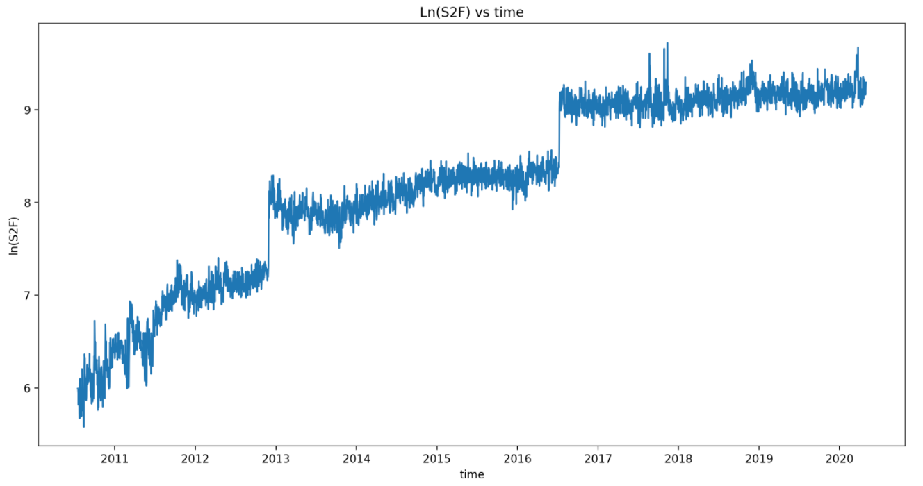
Chart 1: Stock to Flow timeseries
Taken as a whole, the timeseries seems to have both deterministic and stochastic elements. We can see there are three epochs and that each epoch seems to have its own trend. Next to that we also see that there is a clear jump (aka the halving or halvening) between the different epochs. These jumps are referred to as structural breaks in literature. So, we seem to have both a change in trend and intercept at the breaks.
The way I like to think about the series is as follows. Given that the blockreward is known for a certain blockheight, the S2F metric is fully deterministic vs blockheight. To show this please note how the flow evolves as a function of blockheight.
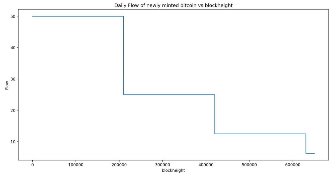
Chart 2: Flow of bitcoin vs bitcoin blockheight
Now look at both supply and stock to flow vs blockheight.
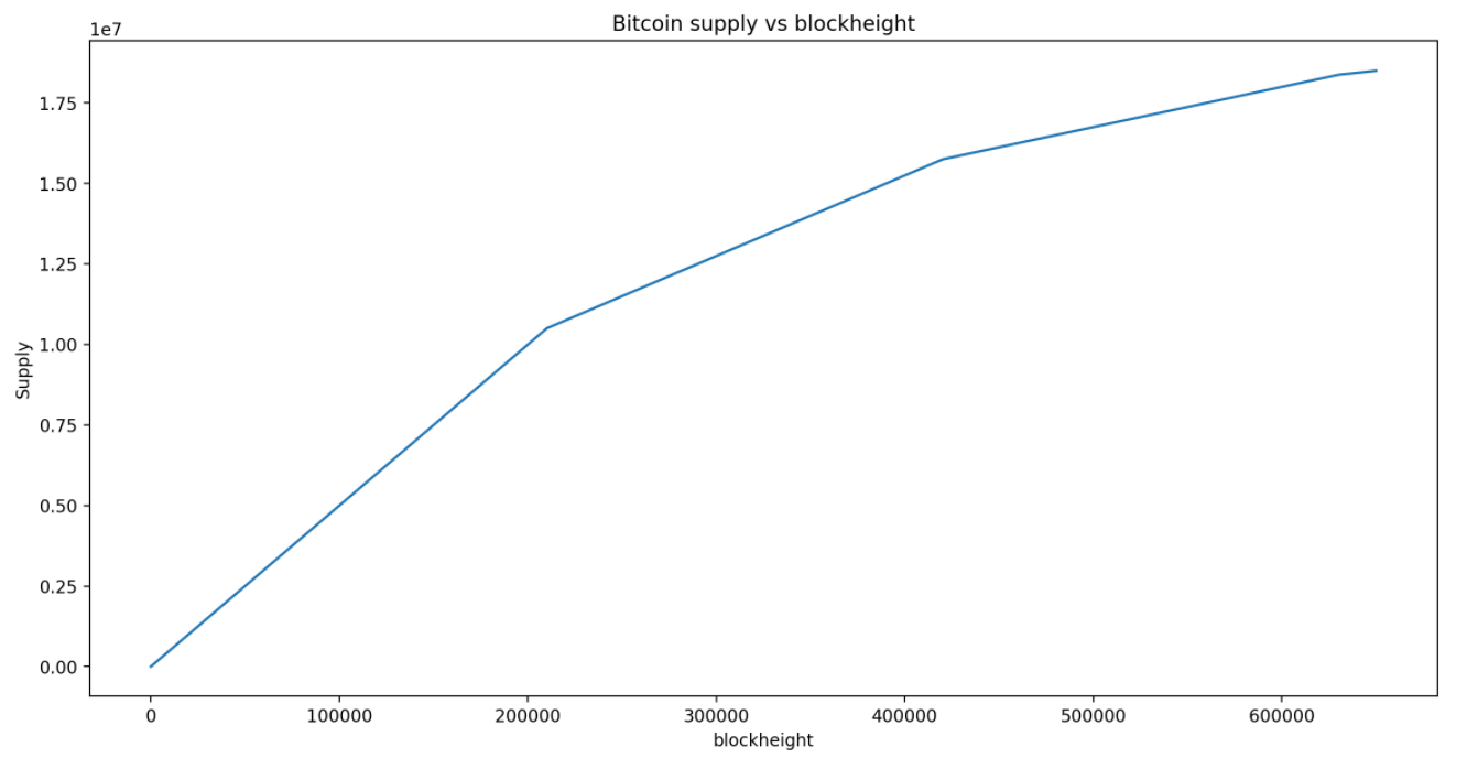
Chart 3: Bitcoin supply vs bitcoin blockheight
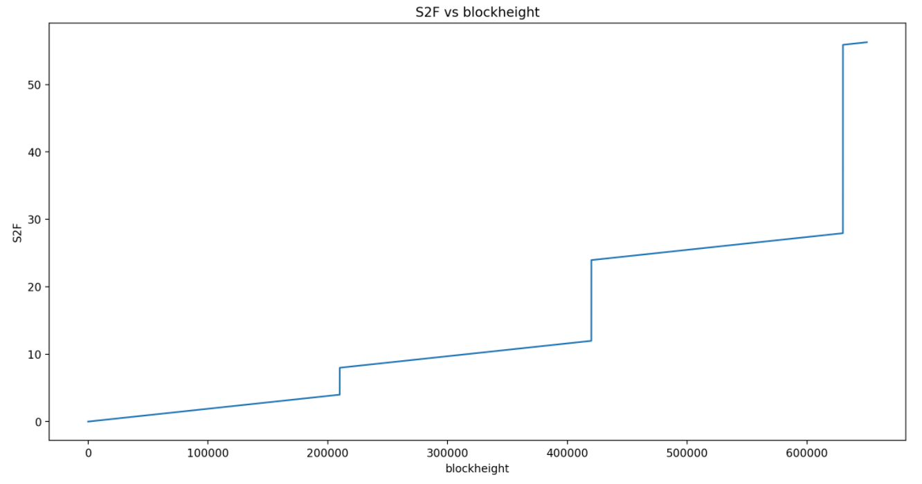
Chart 4: Bitcoin S2F vs bitcoin blockheight
All these evolutions over blockheight are fully deterministic. The stochasticity we observe in the timeseries of S2F vs time comes from the uncertainty in the interarrival time for each block. I took a sample of 10.000 inter arrival times and had a look into the distribution.
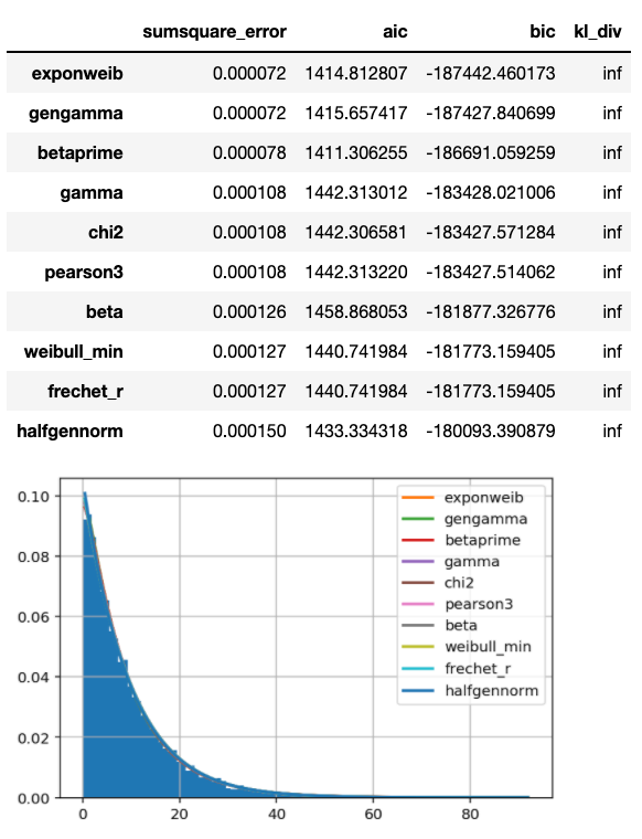
Distribution Fitting of blocktimes for bitcoin
The deviation in the interarrival times causes the S2F metric over time to show some stochasticity. If miners would mine new blocks exactly every 10 minutes, then S2F over time would actually be fully deterministic. But this is how S2F looks vs time.
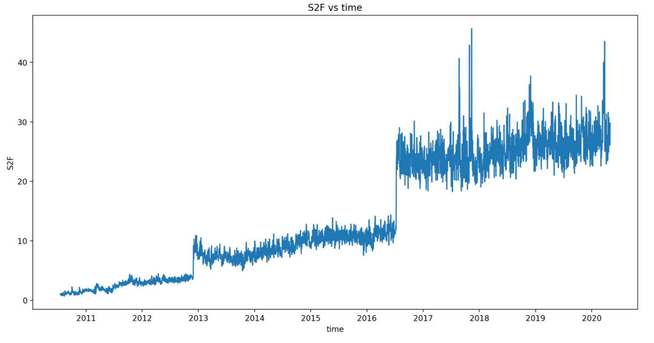
Chart 5: Stock-to-flow over time
Let’s have a closer look at the distribution of daily flow per reward era.
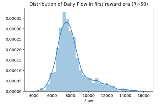
Chart 6: Distribution of daily flow in first reward era
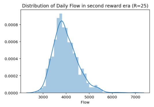
Chart 7: Distribution of daily flow in second reward era
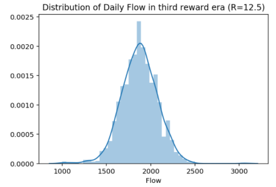
Chart 8: Distribution of daily flow in third reward era
It’s exactly this variance in Flow that you’ll see back in the day to day change of the S2F metric as well.
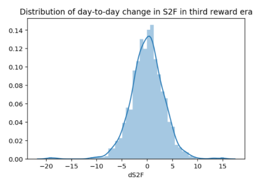
Chart 9: Distribution of day-to-day change in S2F in third reward era
So now we know exactly where the variance is coming from and how it looks like. Given all the analysis above, I think there is enough reason to assume that S2F has 2 deterministic elements;
- a deterministic intercept for every reward era
- a deterministic trend for every reward era
This would leave us with a model for S2F that looks like:

Eqn 1: stochastic model with deterministic elements to describe S2F over time
In the above model alpha is the reward era dependent intercept and beta represents the reward era dependent trend. Epsilon represents the noise resulting from variance in blocktimes.
After correcting for the deterministic components, we are only left with a most likely stationary process; epsilon.
What does this mean for cointegration?
In order for two variables to be cointegrated, we require two time series with an equal order of integration. In the previous analysis, I showed bitcoins price is first order integrated, and that still stands. Bitcoin doesn’t show any deterministic elements in the evolution of price over time.
For the S2F timeseries I did not correct for the deterministic elements in the series in my earlier work, which according to Engle and Granger should have been corrected for before determining the order of integration. If we strictly follow Engle and Grangers theory and the Wold decomposition theorem, we see that after correction for deterministic elements in the timeseries, we are left with a most likely stationary process.
After correction for the deterministic elements, S2F turns into a I(0) timeseries, while price still is a I(1) timeseries. In this case cointegration as defined by Engle and Granger is impossible, as per definition both processes should have the same order of integration.
Conclusion
The concept of cointegration once saved the by now famous stock-to-flow model from a potential spurious relation between S2F and bitcoin price and is now shown to be improperly applied in among others my earlier work. This means that my earlier work “Reviewing “Modelling Bitcoin’s Value with Scarcity” — Part II: The hunt for cointegration”is invalidated; there is no such thing as cointegration between ln(S2F) and ln(price).
So, now that cointegration is off the table for the model as is, we are no longer able to prove the relation between S2F and bitcoin price isn’t spurious. This doesn’t mean that the current model and all the metrics around it are useless, but I’d consider them as additional equipment in your Technical Analysis toolkit. It’s up to you whether you deem that useful or not.
A final note
I’m not concluding there is no relation between bitcoins price and scarcity. I still think there is a connection between the scarcity of bitcoin and price. I am concluding that we can no longer prove that the S2F model as laid out by PlanB is the model that is able to describe this relation while respecting the definitions and assumptions of the applied statistical concepts.