The Intelligent Bitcoin Miner, Part I.

If you find WORDS helpful, Bitcoin donations are unnecessary but appreciated. Our goal is to spread and preserve Bitcoin writings for future generations. Read more.

Make a Donation

---

The Intelligent Bitcoin Miner, Part I.

By Leo Zhang, Jack Koehler, and David Cai - general mining Research

Posted November 22, 2020

This article is a collaboration with General Mining Research, a Singapore based hashpower-focused company, who invests and trades hashpower of cryptocurrency networks, as well as derivatives. GMR supports our work by providing proprietary machine market data, as well as hashrate growth predictions over the next few months based on sales projections aggregated from manufacturers.

“You will be much more in control, if you realize how much you are not in control.”

― Benjamin Graham,The Intelligent Investor

The valuation of hashpower is one of the oldest and most arcane topics in the mining world. Several prior academic papers and industry research have explored the economic and game theoretic aspects of proof-of-work, but most of them oversimplify or make unrealistic assumptions about how the hashpower market works in practice. 

In this paper, we illustrate that operating hashpower is akin to managing a portfolio, and the difficulties of reflecting the aspects of portfolio in the pricing of hashpower. We walk through how the popular pricing mechanism works, and the flaws of the current valuation heuristics. We parametrize a hashpower portfolio, and show how the outcome changes as we test a broad range of assumptions. As a coda, we argue that the importance of valuation framework is more than just a theoretical exercise, but a foundational step in developing a proper risk management practice for the hashpower industry.

The Fair Value of Hashpower

Why run a mining operation when you can purchase coins on the open market?

This is the most common reaction when someone first hears about mining. It’s no secret that it was the outsize financial return that spurred the initial interest in mining and accelerated its growth into a billion-dollar behemoth. A successful miner is able to produce Bitcoin at a cost lower than the spot price, and can accordingly build a position at a steep discount compared to purchasing on the open market. 

However, the low cost-of-production is by no means permanent. Over the years, competition has been heating up, and the market cycle is becoming too obscure to predict. The “discount” that the miners have gotten so spoiled with can deteriorate into painful loss any moment. In today’s market, is mining still more profitable than purchasing on the open market? Given the number of variables involved, it’s futile to attempt at a timeless generalization. However, we can break down the market cycle into several archetypal phases, and observe how the profitability of common mining and trading strategies evolve in each phase. 

We’ll begin with 2018, a miserable year for most miners. In the previous article, we describe the first three quarters as the Inventory Flush phase of a mining cycle, where coin price drops while network hashpower continues to increase. 

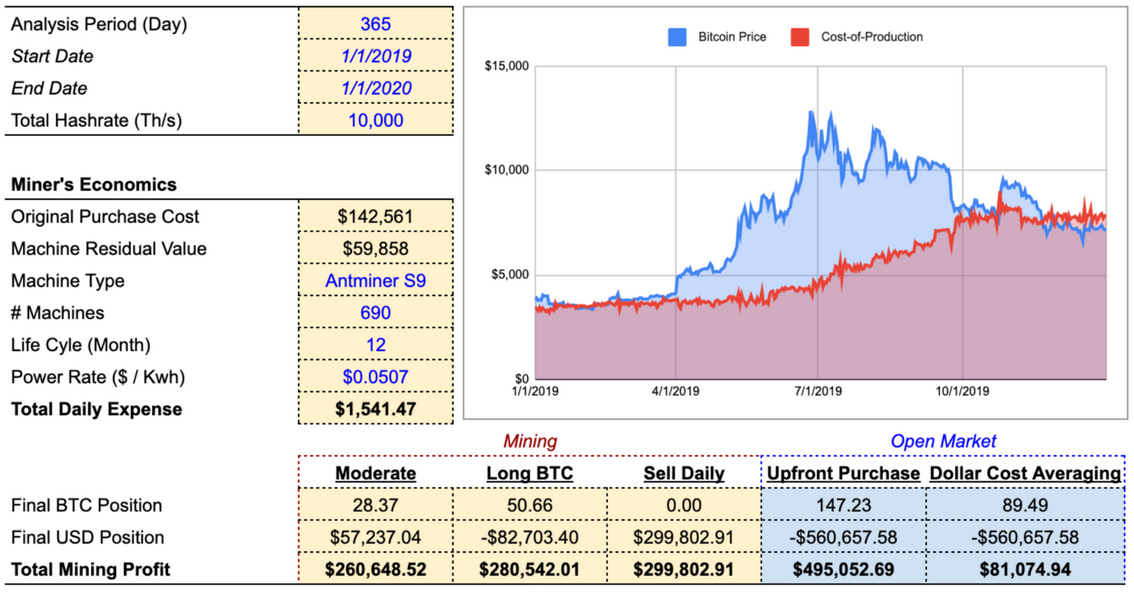
Hypothetically, a miner that purchased 10 Ph/s of Antminer S9 at the beginning of the year would have spent a total of $1.85MM spent on 690 units given the unit price at the time of $2,675 per machine. Assuming the machines linearly depreciated over 24 months, and the miner’s all-in electricity cost was $0.0507 per KwH (industry-wide average rate in China, courtesy of GMR) , we can backtest the performances of three common strategies: 

1. Moderate: the miner sells enough coins to cover the daily power bill ($941.38) as well as the daily depreciation ($2,563.54). If the mining revenue of the day is less than the total expense ($3,709.01), then only sell enough to cover the power bill. Everything else remains in BTC position. 
2. Long BTC: the miner sells just enough to cover the daily power bill ($941.38), leaving all remaining coins in a long position. 
3. Sell Daily: the miner immediately sells all coins into USD. The only goal is to arbitrage the difference between spot price and cost-of-production. Worth noting that this strategy is not tax efficient and incurs constant market slippage. For modeling simplicity we do not take these factors into consideration. 

Next, we compare the performances of the mining strategies against open market purchases. We consider two simple strategies:

1. Upfront Purchase: On the same day as the mining valuation period starts (1/1/2018), buy coins whose notional is equivalent to the total capex + yearly opex ($1,845,750 + $941.38*365) at the spot of that day ($13,465), and hodl till the end of the valuation period. For the sake of simplicity, we will not factor in the significant amount of slippage incurred by purchasing this quantity of bitcoin. 
2. Dollar Cost Averaging: Spend the same notional as mining capex + yearly opex, but purchase a uniform notional ($2.26MM / 365) of coins everyday throughout the valuation period.

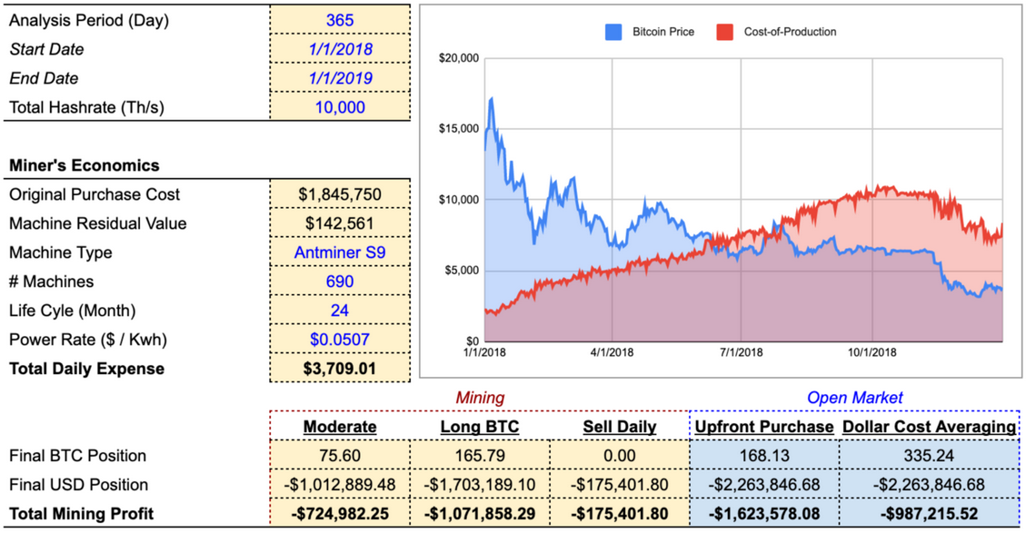
Over the course of the year, daily cost-of-production per coin ($3,709.01 expense divided by the number of coins mined on that day) surpassed market price around July, and kept climbing in the second half of the year, rendering the miner unprofitable for an extended period of time. As we can see from the result, after a year of bear market, the Sell Daily strategy lost the least amount, and the Long BTC strategy took the biggest hit. 

This is because Sell Daily is the only strategy that has no unrealized PnL. Every other strategy has long positions to various extent. During the Inventory Flushphase where mining revenue continuously decreases, the unrealized position is very likely to result in a loss at the end of the valuation period. 

In practice, sensible miners would have turned off the machines after mining at loss for such a long period of time. If the miner had shut down the operation at the end of June, their loss would have been a lot smaller. If the miner were using the Sell Daily strategy, the miner would even have made a profit:

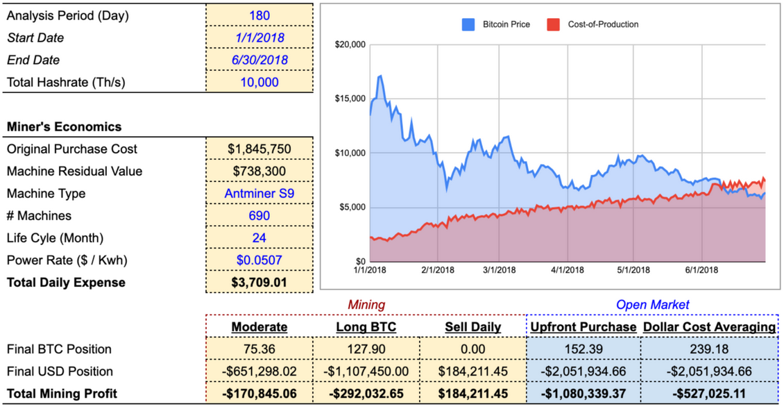
The Moderate and Long BTC strategies would have remained unprofitable, albeit to a lesser extent than open market purchases. The loss primarily stems from capital expenditure of the machines. The miner bought them at $1.84MM, but could only resell them for $738K (not including transaction slippage, transportation, and tax). The gains from the Bitcoin mined did not make up for the hardware depreciation. 

In both examples, Sell Daily appears to be the safest strategy. What happens in an opposite phase in the market cycle, where mining revenue continuously increases?

After the Shakeout phase at the end of 2018, the first half of 2019 turned out to be quite festive for miners. Performing the same analysis but from 1/1/19 to 6/30/19, we can see that Sell Daily would have been the least profitable, whereas the aggressive strategies, Long BTC and Upfront Purchase, would have done more than 50% better than the defensive strategy.

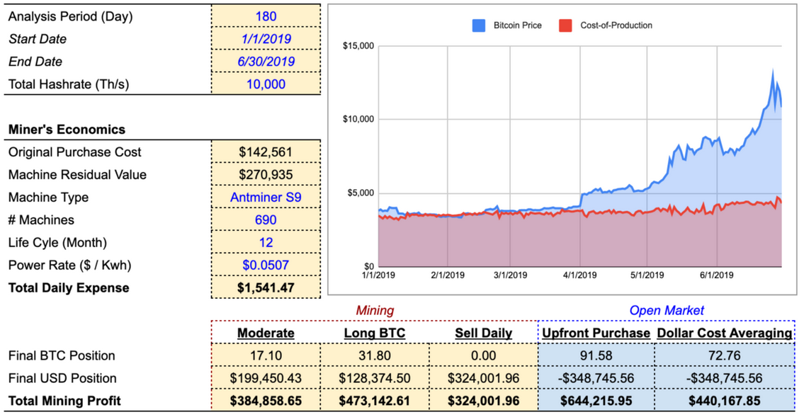
*Life Cycle adjusted to 12 months at the beginning of 2019.

It’s easy to identify the winning strategy with the benefit of hindsight. It takes conviction and deep understanding of the macro conditions to adopt the aggressive strategies when the overall market has been depressed for a while. This especially the case for Upfront Purchase, which requires deploying all the capital on day one. 

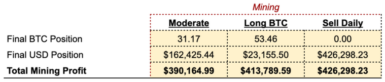
Mid-2019 was also a transition period where new generation machines became available. It’s common for miners to sell old machines to rotate into more efficient models. In this example, the miners could actually sell the machines at prices higher than their purchase price thanks to the raging price rally. 

Hypothetically, if the miner sold all 690 units of Antminer and used the $271k proceeds to purchase new Whatsminer M20 for the second half of the year:  

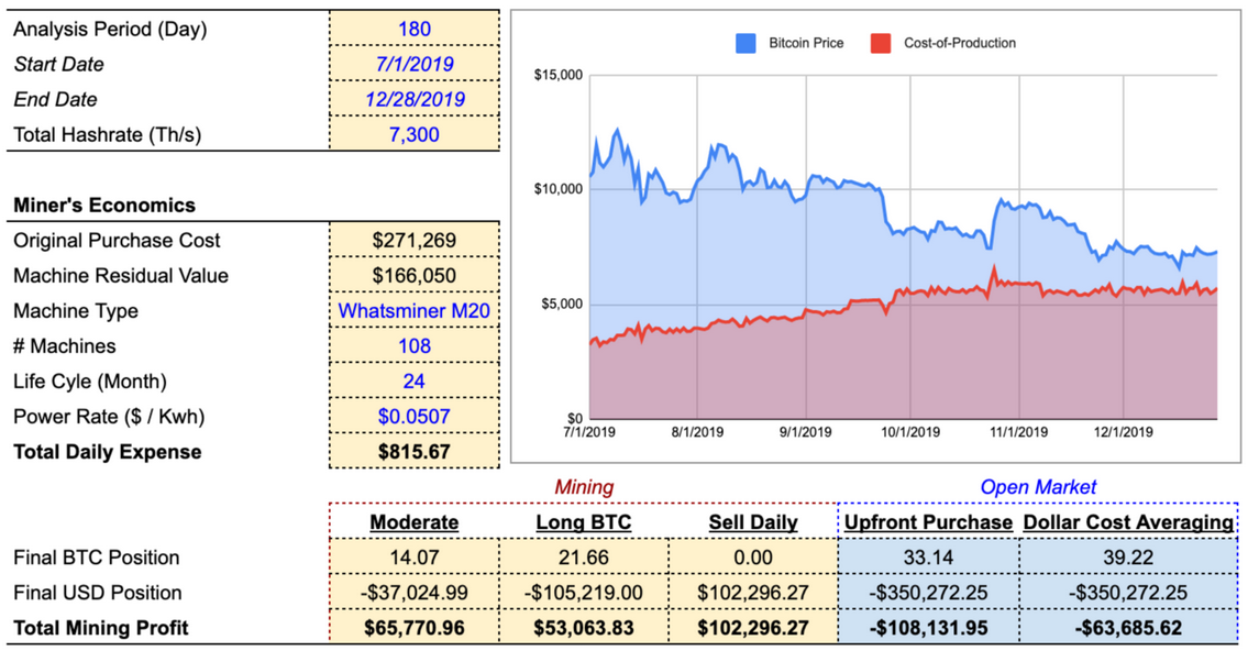
For the entire year of 2019, the miner would’ve made:

Whereas if the miner hadn’t rotated machines, and continued to mine with Antminer S9 for the entire year, they would have left a lot of money on the table:

In practice, miners are not tied to a specific modus operandi for the entire mining period. They have the flexibility to change the strategy whenever they think the market trend is shifting. In addition, they can complement mining with trading strategies, or lend out the coins to enhance the yields on the inventory, for instance, the miner can sell and capture profits on days mining profit exceeds cost-of-production, and buy coins on open market on days mining profit is lower than cost-of-production. Using the right combination of strategies during different stages of the mining cycle has a significant impact on the outcome. The purpose of this exercise is not to come up with a generalized winning strategy, or to prove mining is strictly better than purchasing coins, but to illustrate that managing a mining operation is essentially managing a portfolio.

These represent the simplest and most common mining strategies. A lazy miner who only uses one simple strategy throughout all market cycles will extract a different amount of value from hashpower compared to a miner who actively employs multiple strategies. There is an infinite amount of hashpower management strategies, but the manufacturer is going to charge the same price for the machine regardless of the buyer’s strategy. Though price is a realized data point, value depends on the user. Ideally, the price of the machines should represent an average of the distribution of the values of all available strategies, but that is not possible. So how does the hashpower industry price machines? What does the price of hashpower represent exactly? More importantly, how should miners value hashpower in a way that fits their own circumstances best?

Hashpower Pricing Heuristics 

In today’s market, the pricing of hashpower is dominated by hardware manufacturers such as Bitmain, MicroBT, and Canaan. They are the only supplier of new hardware, they have full control over the initial issuance of machines that produce hashpower. The manufacturers’ first priority is to cover their expenses, which has less to do with the cryptocurrency market and more with supply chain management. The sale price of their product can be adjusted according to market demand, provided it guarantees a certain margin over its cost of production. Sometimes manufacturers artificially suppress the pricing to outsell their competitors. In short, manufacturers’ pricing does not represent the theoretical fair value of hashpower. It is mixed with business decisions that reflect the state of their own companies. 

In part 1 of Alchemy of Hashpower, we discussed that the most popular metric for hashpower pricing is static-days-to-breakeven (DBE). It measures how many days it takes to break even on the machine purchase given the current snapshot price, difficulty, fee, and all-in opex. Every miner has a different DBE on the same machine because every miner runs operations differently. Miners calculate their DBE based on their own all-in cost per KwH and capacity. Manufacturers cannot take all miners’ costs into consideration, so the starting point of their DBE is always a market-wide average all-in cost. This figure is a very rough estimate, since the necessary data is extremely challenging to collect and underlying conditions are constantly changing. Miners with different capacity and cost structure come and go. Manufacturers do this exercise with their best guess on all-in cost, and set the price of the machines based on a reasonable range of the DBE.

But what is the industry-wide all-in cost that they use as the input? We can reverse engineer it with historical machine price data. 

Using the Discounted Cash Flow method, we can backtest historical machine prices to find the underlying assumptions when the manufacturers priced the machines. For example, the retail price for an Antminer S9 in January 2018 was $2,675. 

Assuming an Antminer S9 life cycle of 24 months, we can map out the historical revenue of a single machine:

Next, we reverse-engineer an all-in cost such that the sum of all the present values of each day’s free cash flow equals the purchase price. Assuming an annualized weighted average cost-of-capital (WACC) of 12.5%, we have:

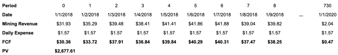
In order to achieve $1.57 daily expense, the all-in electricity cost for an S9 needs to be $1.57 / 24 / 1.365 = $0.048 per KwH. This means that unless the miner had access to $0.048 per KwH all-in cost or lower, the miner would’ve purchased the machine at a premium. The result above is calculated using Strategy 3, Sell Daily. Replicating the analysis with other strategies, Strategy 1 Moderate requires $0.017 per KwH all-in cost, and Strategy 2 Long BTC requires a $0.01 per KwH all-in cost. This means that in practice the actual “breakeven” all-in rate was within the range of $0.01-$0.048 per KwH.

This is drastically lower than the rate available to most miners at the beginning of 2018. Intuitively that makes sense. At that time the Bitcoin price had just reached all-time-high, the network difficulty was just beginning to catch-up, and S9 was the best machine on the market at that time. The ultimate determinant of price is still the supply and demand.

Applying the same method to machine prices at other points in time, the table below would be the “breakeven” all-in cost for miners. Here the all-in cost is the mean of all three strategies:

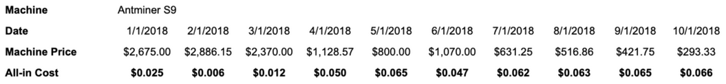
From a different perspective, if the industry-wide all-in cost was $0.0507 per KwH, what would be the fair value of the machines at the time? Again, the Fair Price here is the mean of all three strategies:

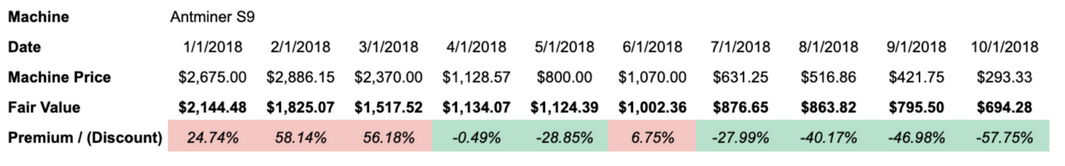
*Premium/ Discount is Machine Price over Fair Value__(Data source: hashrateindex.com)

Note that this analysis does not take the changes in industry-wide average rate or WACC into calculation, since the precise industry-wide rate and WACC are difficult to estimate.

The point of this analysis is not to find the absolute fair value. As discussed, the fair value is not the same for every miner due to the different operating expenses as well as different strategies. However, even with an assumed industry-wide average rate, we can show how wildly inefficient the machine pricing is. During the bull market the manufacturers significantly overpriced the machines, and during the down markets the manufacturers were forced to liquidate the machines at a discount. This is aligned with empirical evidence we see in the mining market. When price rallies fast, the machine prices sometimes go up faster than the coin price. This behavior diverges from fundamentals, which indicate that machine prices should rise more slowly given the expectation of a future increase in network difficulty. At the end of the day the pricing of the machines is driven by supply and demand, and the hashpower market is highly illiquid.

By backtesting the historical machine prices we can see that pricing heuristics based on Static Days-to-Breakeven are insufficient in capturing the volatility of mining profitability. In order to assess the fair value of the machines today, we need to model mining profitability on a forward-looking basis, with tools or frameworks that can capture the wild fluctuations of the outcomes.

A more advanced approach is to treat hashpower as a form of call option. The principle of this approach starts with treating the mining revenue of a machine as the underlying asset. There are three constituents for mining revenue: price, difficulty, and fees. A call option on Bitcoin price is arcane enough, but a derivative instrument that encapsulates these three elements is far more complex. Describing the Black-Scholes theory for options on multiple underlying assets is straightforward: the additional considerations are the correlated random walks and the corresponding multi-factor version of Ito’s Lemma. However, establishing the correlation matrix between the three variables is a daunting task.

As discussed in the Alchemy of Hashpower series, price and hashpower have a cross-correlation with a varying lag. Due to the reaction delay, when examining the relation between hashpower and price in a short time window, the correlation is de minimis. Hence, it’s tempting to simply model hashrate paths as a process completely independent of price. However, financially hashpower is a derivative of Bitcoin, and on a long enough time scale, the two time-series are positively correlated. On the other hand, transaction fees dynamics is even harder to model. While intuitively on some level transaction fees are connected to price and (inversely) to network hashrate, it is predominantly driven by on-chain activities, which is an exogenous factor. This is why the correlation matrix is not going to have meaningful results.

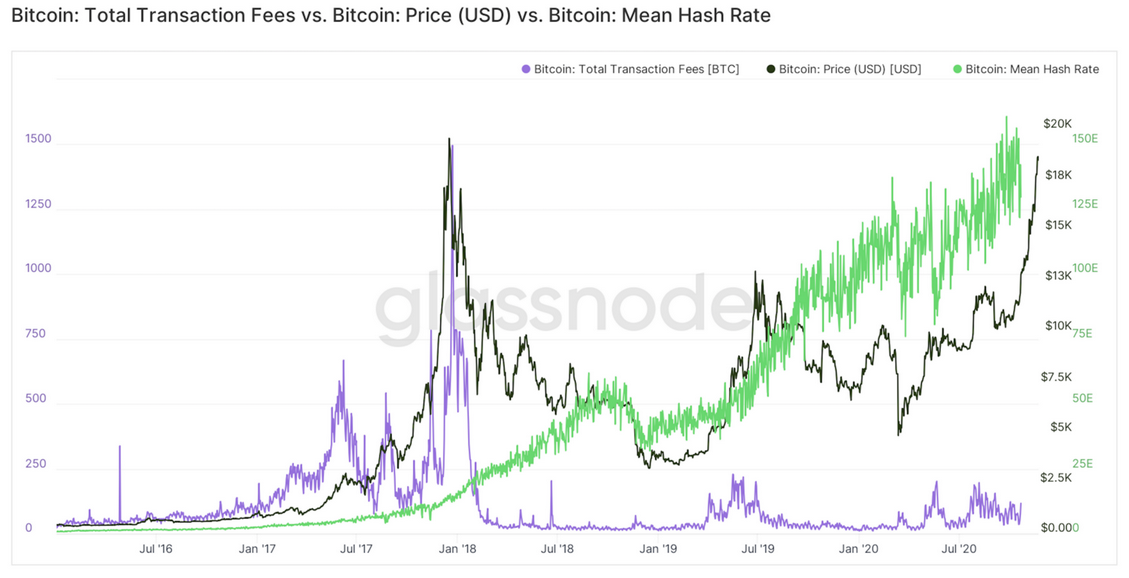
(Source: Glassnode)

But once the assumptions on the distribution of the underlyings have been made, pricing hashpower in a period N is equivalent to pricing a series of zero-strike European call options with daily expiry. In other words, as long as the machine is on, the hashpower is a contract that exercises everyday, and converts into the underlying asset, which is the mining revenue. The cost of the contract is the depreciation of the hardware, plus the operating expenses. The option premium of the entire bundle should in theory be the price of the machine plus the present value of all the operating expenses incurred during period N.

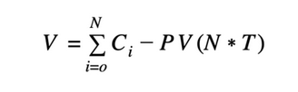
Where:

• V is the fair value of the machine.
• Ci is the call option value with mining revenue as underlying, with expiration on day i.
• T is the daily operating expense.

There is a critical flaw with this approach. Using this formula, the contract on day i and on day i-1 are valued independently. In reality, the payoff on day i-1 should set the initial condition for the contract expiring on the next day. Any hashpower valuation approach based on options pricing and simply sums up all trials in the period will face this path-dependence issue. Every trial will be a disjoint assessment.

Valuation with Numerical Methods

Path-dependence is not an issue with numerical methods. Rather than valuing each day with 10,000 trials we are using the same 10,000 trials across all of them. Monte Carlo simulation is useful in modeling complex dynamics by generating random numbers. The expected payoff in a risk-neutral world is calculated using a sampling procedure. It is then discounted at the risk-free interest rate. With Monte Carlo methods, we are able to simulate the mining profitability of the latest-generation machines in the next two years, and compare their fair value against their prices on the market today.

As a first step we need to make some assumptions on the trajectory of price. A numerous studies argue that jump-diffusion is the most suitable in describing Bitcoin price distribution. We use a jump-diffusion model to simulate 10,000 possible price runs over the next two years. In a stochastic simulation, every run takes a different path.

A jump-diffusion model has two basic parts:  the diffusion (geometric Brownian motion) and the jumps (usually Poisson distribution). For modeling simplicity, we assume that there is a threshold probability for the jumps. When jumps are triggered, the magnitude follows a normal distribution. 

Calibrating based on historical price data, we use the following as the parameters for the model:

• Constant drift: 0.10%
• Standard deviation of drift: 2.50%
• Jump probability: 5.00%
• Jump mean: 0.10%
• Jump standard deviation: 5.00%

In addition to coin price, we need to project the network hashpower as well to calculate mining revenue. Modeling hashpower is more complicated than price trajectory because not every unit of hashpower is the same. While every miner on the network is computing hashes for the same algorithm, the amount of power consumed varies by machine. The simplified model of the current network hashrate abstracts away the presence of several hardware efficiency classes, each of which behaves differently as the market evolves.  Stratifying our model by efficiency class shows us the composition of machines on the market, and therefore allows us to roughly predict how they would evolve over time.

Unlike price data, mining information is extremely challenging to collect. The only way to approach this is to interview as many miners, distributors, and manufacturers as possible. David from General Mining Research surveyed the major manufacturers and distributors in China, and came up with the following estimate of the market composition as of 11/1/2020:

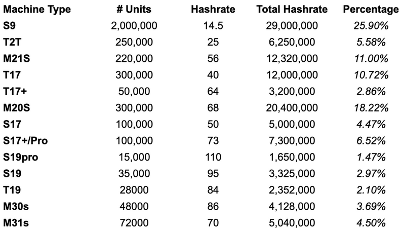
(Source: Proprietary data provided by GMR)

The snapshot serves as the basis for the initial condition of the projection model. Using an estimated industry-wide average all-in electricity rate, we can calculate the breakeven threshold for each layer, and understand roughly how many machines will likely drop should the price fall below the breakeven. Using $0.0507 per KwH as the estimated all-in rate, we can map out four possible scenarios based on different price levels:

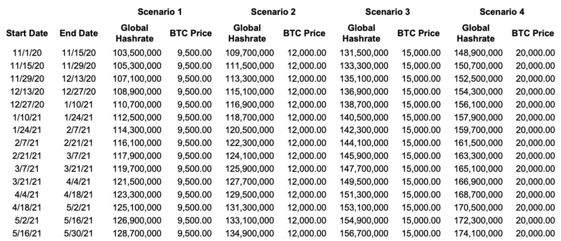
(Source: Proprietary data provided by GMR)

Note that this only provides a baseline view of the hashrate projection. Old, marginally-economical machines sourced via secondary markets may come online and manufacturers may accelerate new production if there is a drastic rally in price.

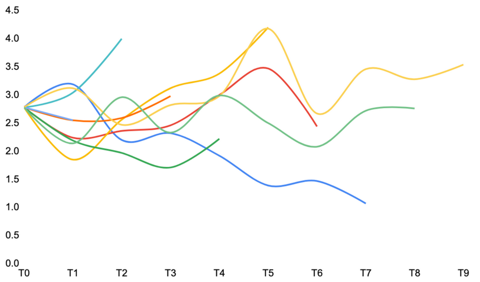
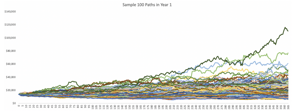
Based on the scenarios above, we can find a linear function y=4,544x + 6e07 to describe the relation between price and the network hashpower. For simplicity, we assume that for the next six months, hashrate growth follows the function of a 14-day average Bitcoin price with a drift term dW. We set 2.5% mean, and 5% standard deviation as the parameters of the drift term. In addition, based on our estimate of machine sales from manufacturers, we assume hashrate grows by 200 Ph/s a day for the next six months. We mimic the hardware reaction delay by incorporating a constant 20-day reaction delay. This means that hashrate only reacts to price action that at least happened 20 days ago. The full function:

Sample trajectories look like the following:

In reality, the relationship between hashpower and price is a messy and complex entanglement. Using a linear function to describe it is like projecting a chaotic system onto a low-dimensional subspace. There are many ways that the function can break. This is the same problem that we describe about the correlation matrix in the option pricing methods. However, this construction allows us to easily incorporate the lag time, and therefore is a significant improvement over assuming hashpower and price as two completely independent distribution. This makes the projection easier to manage.

To further improve our estimates, we can use a Markov Chain Monte Carlo model. Unlike Monte Carlo draws independent samples from the distribution, Markov Chain Monte Carlo draws samples where the next sample is dependent on the existing sample. This addresses multi-dimensional problems better than a generic Monte Carlo simulation. The exact construction of the algorithm is beyond the scope of this article.

Once we have the projections for price and hashrate in the next two years, we can calculate the mining profitability the same way we ran the backtests on the historical hashpower prices. Compared to two years ago, where crypto-backed lending activities were sparse, the lending market today has grown into a massive industry. Collateralize lending is one of the most common services that miners frequently rely on. Evaluating the WACC today, the rate should improve noticeably. We can lower it to 10% instead of the 12.5% in the 2018 analysis.

Using a $0.0507 / KwH all-in cost, and a 10% discount rate, we can generate a distribution of the fair values. The final result is the average of all 10,000 trials. Additionally, we assume that after two years, Antminer S19 Pro and Whatsminer M30s still retain 20% of residual value.

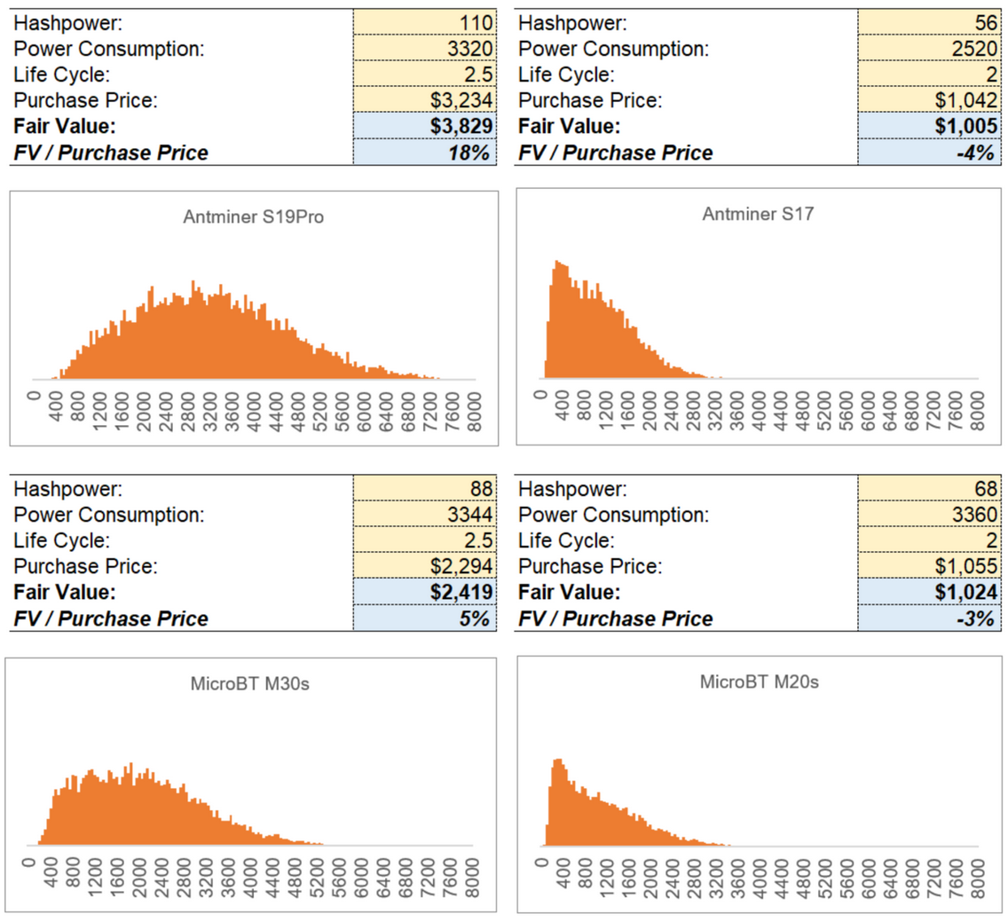
Needless to say, this should not be a final verdict on whether the machines are overpriced or underpriced. The mean and standard deviations in the price distribution, the function between hashpower and price, lag time, all-in cost, discount rate, and residual value are all factors that can drastically affect the outcome of this evaluation. For instance, running the simulation with $0.07 per KwH and with $0.03 per KwH all-in cost:

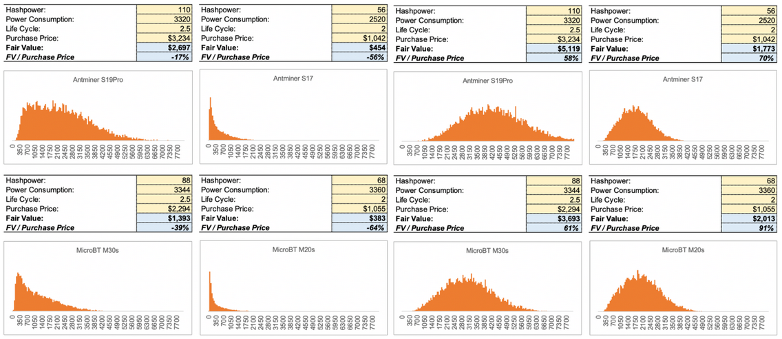
We can see that when the all-in cost is high (left), the prices of the more efficient machines (Antminer S19 and Whatsminer M30s) are closer to their fair value than the lower tier machines. When the all-in cost is low (right), the pricings of the less efficient machines (Antminer S17 and Whatsminer M20s) are more favorable. This shows that if the all-in expense is competitive enough, the miner can benefit from operating less efficient machines.

In our model we built a switch that turns off the machines if the mining revenue is consistently below expenses for 14 days. In the real world, miners don’t frequently turn machines on and off based on short-term profitability. Most of the time miners have agreements with the datacenter host that they need to consume a minimal amount of power every month. Even after profitability drops below zero, most miners tend to wait for a downward trend to confirm before taking actions. Due to the labor-intensive nature of datacenter operations, and the illiquidity of machine market, miners are forced to observe longer term trends instead of short term price actions. In recent years, the rise in the volume of lending service providers also strengthened miners’ ability to endure through winters. Miners can collateralize their coins or machines to borrow fiat to pay for expenses, rather than selling a great quantity of coins. Nonetheless, this is a theoretical lower bound on mining loss. Miners cannot lose more than the capital expenditure plus the cumulative operating expense.

Like call options, the more volatile the underlying index is, the higher the theoretical value of the instrument. We can see how the results change as the parameters of the jump-diffusion model changes. When volatility is suppressed, the theoretical value of the machines drastically decreases. When volatility is high, the theoretical value rapidly increases:

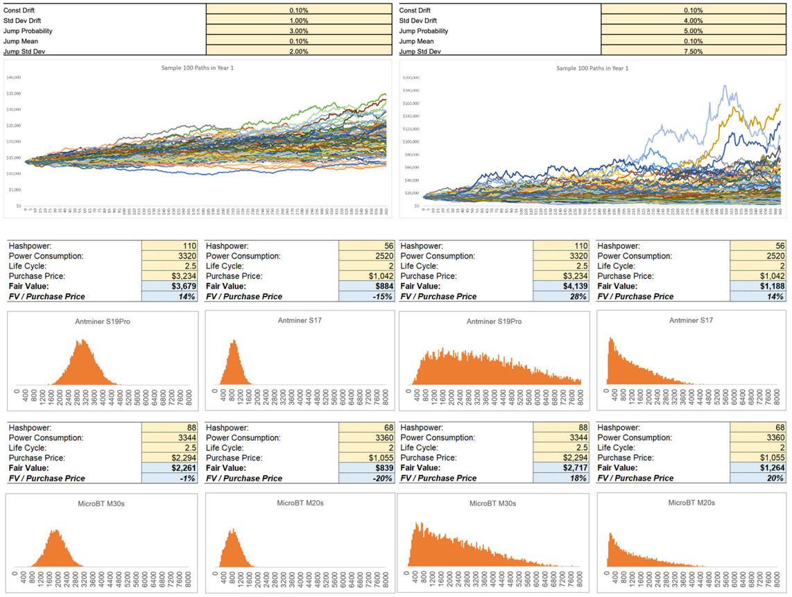
*Based on $0.0507 per KwH all-in cost

This analysis is based on Strategy 3 Sell Daily. Same as the backtesting analysis, the fair value that can be “unlocked” by running hashpower is within the range of FV(Strategy 1, Strategy 2, Strategy 3). Given that the Monte Carlo simulates 10,000 paths, each with a very different path, running one strategy alone should be sufficient to cover every type of market phase.

A Future without Block Rewards

Another variable that has a significant impact on mining revenue is the fees. Assume fees grows linearly by 5% and 10% a year, fair value of the machines would noticeably increase:

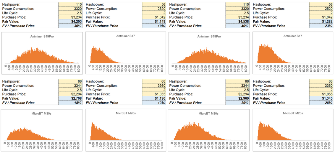
*Based on $0.0507 per KwH all-in cost

In reality the fee trend is much more sporadic, and its connection to other endogenous variables is less obvious. Modeling fee trends requires an entirely separate distribution. In addition, there are many ways to improve the accuracy:

1. As discussed, use Markov Chain Monte Carlo to alleviate the curse of dimensionality, 
2. Introduce dynamic lag based on the four archetypal market cycles, use a poisson process to model the jumps.
3. Use a hashrate-weighted average all-in cost instead of industry-wide median cost. 
4. Use statistical methods to calibrate the parameters
5. Use machine learning tools to describe the relationship between hashpower and price. 
6. Incorporate fee projection in mining revenue calculation. 
7. Adopt agent-based simulation for miner behaviors. Agent-based modeling is a technique for modeling complex systems to gain a deeper understanding of system behavior. It is widely used in high-frequency trading, or smart contract risk analysis. Under this framework, every miner is a “user” with different strategies and different cost basis. We can then define some simple reaction types (buy more machines, sell machines, buy more machines but wait for 30 days etc.) and build a library of “user behaviors”. This would allow us to simulate much more complex interactions in the hashpower market. For more background, read about Conway’s Game of Life. 

Myron Scholes said, “all models have faults - that doesn’t mean you can’t use them as tools for making decisions.”

Like the Black-Scholes model, the simulation model is a mechanism that, in trying to reflect the actual world in a short description, simplifies its intricacies. This reduction makes the model usable but simultaneously limits its usefulness. It’s important to understand where its limitations are, and that the simulations only represent possibility not certainty.

Nevertheless, the model is a baseline for users who have already formed a view on the market. Like any forecasting model, the simulation will only be as good as the assumptions the user makes. One uses modeling tools to turn those opinions about the future into an appropriate price today for something that will be exposed to that version of the future.

Why is this important? What’s the point of developing asset pricing theory in a market that is clearly driven by supply and demand?

Valuation is more than just a theoretical exercise. For Bitcoin, once mining becomes completely reliant on fees, competition yields razor-thin margins, and there is not a single element in mining revenue calculation that is predictable, how do we make sure miners keep producing hashpower? The answer is to maintain stability of continuous investments into mining hardware to augment the security budget of the network. This is critical because without enough hashpower, the whole system is susceptible to attacks, rendering Bitcoin’s settlement assurance worthless. A rigorous valuation framework is the first step in testing a broad range of assumptions and market behavior and planning accordingly. Valuation is the foundation of proper risk management for mining institutions that are becoming too-big-to-fail. The purpose of this exercise is to start a dialogue that focuses on this general direction. We will continue working to further our framework for years to come.

---

Subscribe to WORDS

* indicates required

Email Address *

First Name or Nym *