How Does Quantitative Easing (QE) Affect the Price of Bitcoin?

If you find WORDS helpful, Bitcoin donations are unnecessary but appreciated. Our goal is to spread and preserve Bitcoin writings for future generations. Read more.

Make a Donation

---

How Does Quantitative Easing (QE) Affect the Price of Bitcoin?

By Pedro Febrero on Quantum Economics

Posted May 11, 2020

With QE on the rise, is Bitcoin poised to fill the gap?

Since the 2008 financial crisis, expansive monetary policies have barely kept the struggling economy alive. With infinite QE on the rise, the only solution in sight seems to be a return to a hard money standard. Will Bitcoin fill in the gap?

In this article, we aim to explore the impact that quantitative easing (QE) has on the price of Bitcoin. To achieve that goal, we will first look into the effects of massive currency creation, how QE works and why it’s so dangerous in the long-term.

Finally, we’ll connect the dots by showing how QE and other expansive monetary measures have influenced the price of traditional assets and commodities, including bitcoin. We’ll conclude the piece by sharing our thoughts on why the return to a hard-money asset is the long-term solution to this particular economic crisis.

How money differs from currency

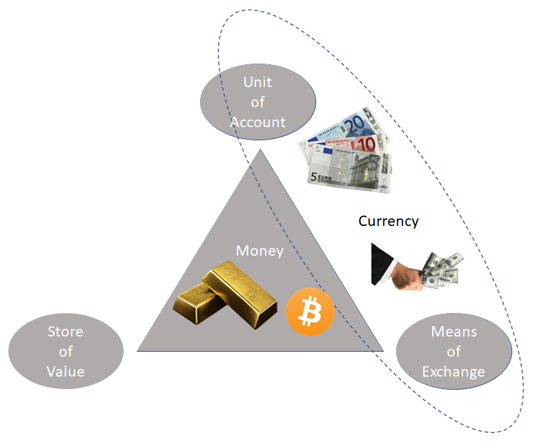Image: Author

A great starting point for our analysis is to discuss the key differences between money and currency. Since we’ll be looking into topics such as hard money and QE, we should, beforehand, briefly explain what makes money different from currency.

Let’s begin by defining what hard money is. Investopedia defines hard money as _“a physical currency, such as coins made out of precious metals including gold, silver or platinum.” _A better definition could perhaps be a form of money that requires a significant amount of energy to produce.

To make the topic more understandable, we’ve developed the picture above. It visualizes what money is (or should be): an asset or commodity, like gold and Bitcoin, that grants its holders the power to store value, exchange value and measure value. Unlike currency, which is great to exchange and measure value, one of money’s most important traits is its ability to store value across long periods of time.

A very good example follows. In ancient Rome, an average centurion soldier would get paid just over 1,077g of gold per year (in sestertii equivalency), which in today’s terms means close to $61,000. In terms of purchasing power, two months’ salary was enough money for a centurion to acquire one year’s worth of bread, much like today, according to some researchers.

Hence, we can conclude that gold has maintained purchasing power since the ancient Roman times.

If we wonder what characteristics allow money to store value during very long periods of time, we come to the conclusion it’s mainly due to skin in the game and proof-of-work. In other words, any commodity that desires to be treated as money should be quite hard to acquire (skin in the game) and should have a limited supply, granted lots of energy is required to mint a new unit (proof-of-work). That’s why gold coins and units of bitcoin are treated as hard money, since they are kinds of currency that are rare and difficult to produce.

Unfortunately, since 1973, the equivalence or standard between currency and money has deteriorated. With the introduction of a global fiat standard, the relationship between the U.S. dollar and gold was relinquished. Effectively, all fiat currencies use the greenback as reserve money, even though those same dollars could be printed at any time by a central bank.

The problem is when economies mix the concept of money and currency. As it is discussed in money theory, base currency should only inflate as much as the real economy requires, and credit money should expand based on hard money reserves. However, since the world’s reserve currency is the U.S. dollar, not gold, central banks could incur a massive expansion of credit through low reserve requirements, simply because paper, or digital numbers on a ledger, aren’t that hard to produce.

Hence, the world entered a downward spiral of nontraditional monetary policies, including quantitative easing, zero interest rates and negative interest rates. The allocation of capital was displaced from the real productive economy into the financial economy, making waves for a period of highly leveraged stock markets.

What is the relation between fiat currency, QE and financial markets?

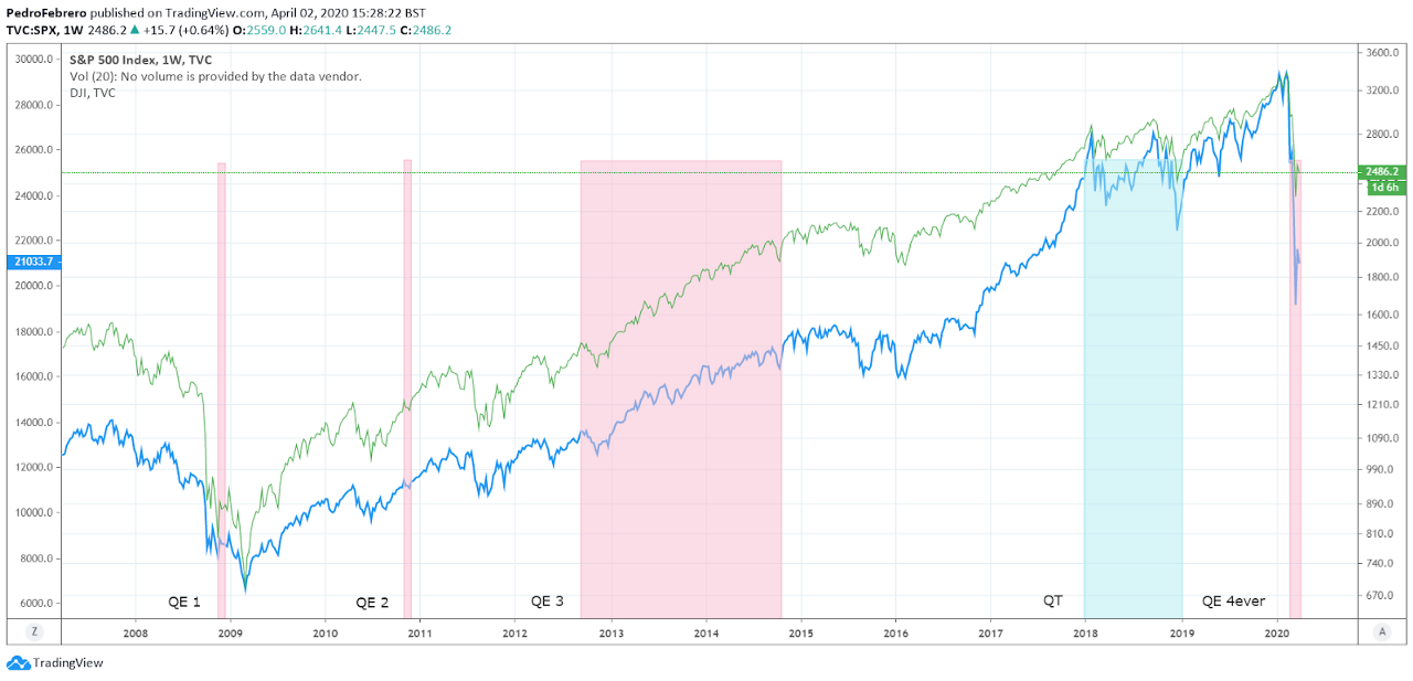This chart shows the S&P 500 and the Dow Jones Industrial Average, 2008–2020 (Source: https://www.tradingview.com/x/O5sPX7vu/)

QE is a brand new monetary policy introduced by central banks worldwide in response to the 2008 financial crisis.

Investopedia describes QE as the following:

“Quantitative easing (QE) is a form of unconventional monetary policy in which a central bank purchases longer-term securities from the open market in order to increase the money supply and encourage lending and investment. Buying these securities adds new money to the economy, and also serves to lower interest rates by bidding up fixed-income securities. It also greatly expands the central bank’s balance sheet”

To give another perspective, we see QE as the tool that allows central banks to purchase assets for free in order to indirectly sponsor corporations into spending. QT, on the other hand, translates to quantitative tightening. This is the exact opposite process, where central banks aim to decrease the assets held, which normally places downward pressure on asset prices.

Without the possibility of creating infinite currency and artificially suppressing interest rates, it would be impossible for central banks to finance their own economies directly. That means government spending would be considerably more restricted to actual money reserves and economic growth, and malinvestment would be costly, since there would be no direct way to bail out failing corporations.

In sum, if governments can’t debase a currency, they can’t print infinite currency, meaning bailouts can only happen through costly debt or increased taxes on income, products or companies. Therefore, had QE not been invented, companies would likely be more careful and would be less likely to misallocate their capital.

Since QE has begun, the global asset markets have skyrocketed in price. The above chart shows precisely what we mean. Did you notice how after each QE round (pink columns), the markets tend to appreciate in value?

From November 2008 to November 2010, between QE 1 and QE 2, both the SPX and the DJI increased, on average, close to 60%. Additionally, from QE 2 to QE 3, which started in September 2012, both markets rose more than 20%.

However, the biggest appreciation took place between September 2012 and 18th February 2020. Both indices increased over 130%, an astonishing accomplishment according to price history. Not surprisingly, during the period of QT, from 2018 until early 2019, both the SPX and DJI had the exact opposite behaviour. Both indexes dropped substantially, between 16% to 20% respectively.

Bitcoin was born amidst the financial crisis, in January 2009, and has gained substantial value since its inception. Undoubtedly, the easing of cash to purchase financial assets may have played a significant role in the optimism surrounding BTC, as we’ll discuss near the end.

Nevertheless, before we dive into Bitcoin, we shall look into how QE influenced the markets in Europe and the United States. Only after we evaluate the impact of QE on asset prices and how it relates to each jurisdiction’s Gross Domestic Product (GDP), we may begin to unravel the answer we seek.

Additionally, in order to make our analysis easy to understand, we’ll look into the effects of the Fed’s and the ECB’s money printing on consumer behaviour by comparing the velocity of money to its total supply.

Hopefully, by the end, we’ll be able to extrapolate the short-term and long-term effects of QE and other expansive monetary policies on the price of Bitcoin.

Now, we’ll start by looking into the ECB’s QE programme, immediately followed by the Fed’s.

Let’s have some fun, shall we?

European Central Bank QE

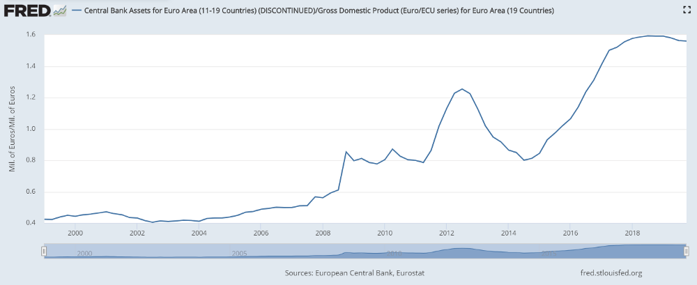This chart shows the total assets held by the ECB. (Source: https://fred.stlouisfed.org/series/ECBASSETS#0)

First, let us dive deep into QE, by looking at the European Central Bank’s (ECB’s) QE program.

Much like in the United States, its QE measures started amidst the 2008 Financial Crisis. The ECB’s first round of purchases took place in Q2 2008, and the institution acquired assets worth more than 20% of the European Union’s total GDP.

A few years later, in late 2011, there was a second round of massive purchases. Essentially, from Q2 2011 until Q2 2012, the ECB bought assets worth 50% of the EU’s total GDP.

By the beginning of 2013, the assets accumulated by the ECB were worth more than 120% of the entire eurozone GDP.

But wait, there’s more.

Soon afterwards, the ECB reduced its balance sheet significantly, reaching the same levels it had in Q2 2011 by mid-2014, at around 80% of total eurozone GDP.

However, the most aggressive buying of assets started soon after. If not, how could they expedite the massive financing of private corporations? Through large scale purchases, the ECB took the total value of the assets it owned from roughly 80% of total eurozone GDP in mid-2014 to around 134% in early 2019.

In other words, while the eurozone GDP was close to €3.5 trillion, assets held by the ECB were valued at €4.7 trillion.

In total, the ECB doubled the value of assets it held in the span of five years.

U.S. Federal Reserve QE

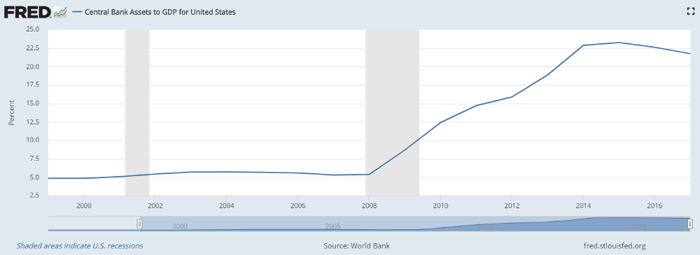This chart shows the total assets held by the Fed. (Source: https://fred.stlouisfed.org/series/DDDI06USA156NWDB)

In the introduction, we already discussed the effects QE has on major stock indices, namely he S&P 500 and the Dow Jones Industrial Average. To complement the initial discussion, we’ll measure the impact the Fed’s QE has on total U.S. GDP, much as we did in the previous section with the ECB.

When QE started in late 2008, assets held by the Fed went from roughly 5% of total U.S. GDP to about 12.5% in early 2010. Soon after, the Fed slowed its pace and only increased its balance sheet by approximately 5% between 2010 and early 2012.

However, things were not looking great for the financial markets and the economy in general. Hence, from 2012 until early 2014, the Fed acquired assets worth more than 7.5% of U.S. GDP.

At its peak, the Fed held assets worth close to 25% of U.S. GDP.

Essentially, the only way markets around the world could appreciate, especially in Europe, the US and Japan — where the BoJ currently holds assets worth over 100% of the total of GDP — was through currency manipulation.

In fact, without the massive repurchasing of global assets, many companies would not be able to survive, for example Boeing, American Airlines or even Hilton. Over a period of two years, Boeing spent $11.7 billion on share repurchases, according to CNN. In addition, American Airlines Group devoted $1.1 billion to such transactions and Hilton announced $2 billion worth of buybacks.

The issue is the fact most of that cash seems to have come directly from the Fed. Curiously, Boeing is now requesting $60 billion in federal assistance, the rest of the airline industry another $50 billion and, finally, the hotel industry is asking for around $150 billion in federal assistance as well.

What this translates into is corporations using near-free cash to provide benefits to shareholders, instead of reinvesting that capital into their business.

Next, we’ll analyse the relationship between the money supply and the velocity of money. Our goal is to predict the current and future behaviour of consumers — if they are either hoarding or spending U.S. dollars — and how that may affect short-term and long-term asset and consumer prices.

The relationship between velocity and supply

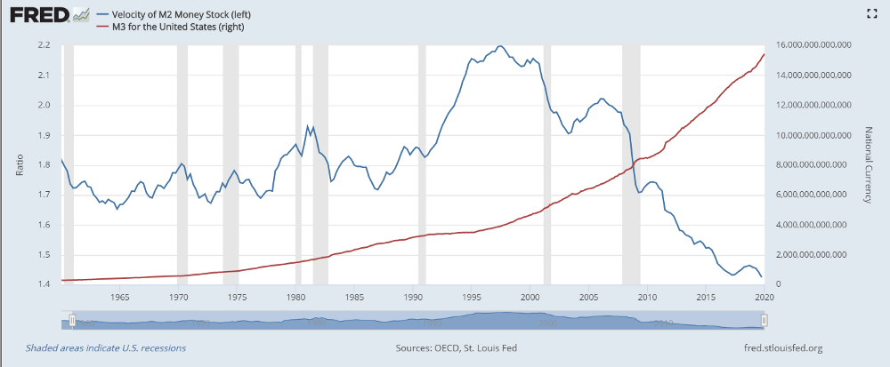This chart shows the velocity of money (left, blue) and the total money supply M3 (right, red). (Source: https://fred.stlouisfed.org/series/MABMM301USM189S#0)

Proponents of Modern Monetary Theory (MMT) and followers of the Keynesian and Chicago schools of economics, like the Bitcoin critic and Nobel Prize winner, Nouriel Roubini, firmly believe it’s possible to print our way out of a financial crisis. However, historical data tells a rather different tale.

Before discussing the chart above, let us summarize our findings so far.

In the previous three sections, we concluded that:

• Europe (ECB) is printing large quantities of currency. At the time of writing, it has confirmed additional QE measures, without an end in sight.
• In 2019, the assets held by the ECB were worth 130% of the total eurozone GDP.
• The United States (Fed) is printing large quantities of currency as well. Much like in Europe, it’s currently breaking all-time highs in terms of available supply. Infinite QE measures have been guaranteed in response to the recent COVID-19 crisis.
• In 2019, the FED held assets totaling 25% of the country’s GDP.
• Since QE 1 started in late 2008, both the SPX and DJI have climbed more than 300%.

Let’s get back to the pretty picture.

The chart above shows the velocity of money compared to the total supply of currency.

The velocity of money (VoM) is measured by looking at how often each unit of currency exchanges hands during a quarter. To calculate the VoM, we simply divide GDP by the money supply. We can see three distinct phases in the chart.

• Between 1950 and 1990, the VoM ratio drifted between 1.7 and 1.9, meaning between 170% to 190% of the entire money supply’s value was being exchanged every quarter.
• In the 1990s, the VoM ratio started rose above 2.0, which means that more than 200% of the entire money supply’s worth was being exchanged on a quarterly basis. The figure stayed above 2.0 for much of the 2000s.
• Finally, starting in the late 2000s, the VoM ratio dropped significantly, falling over 35%. It went from a high of 2.2 to a current low of about 1.44, meaning only around 144% of the entire money supply’s worth is currently being exchanged per quarter.

Hence, we can safely say a smaller percentage of monetary units are being exchanged today than in 1950, which means that either corporations (or people) are hoarding cash because they’re scared, or the number of monetary units has flooded the economy.

Could it be both?

The long-term impact of QE on consumer prices

We concluded in the previous section that less of the money supply is being spent. The downturn started at the eve of the “internet bubble,” in the late 1990s, and VoM continued to fall further until today. There have been a few attempts to recover consumers’ and corporations’ confidence in the economy, but none have succeeded. The problem will only get worse. What do you think will happen when the economy picks up and the saved-up money reenters consumer markets?

To answer that question, we need to take another look at the chart. But now, let’s analyse the increase in money supply (red).

Over the course of almost 50 years, from 1950 until 1998, the money supply increased 13x, from $300 billion to nearly $4 trillion (red line on the chart above). Still, what happened next is astonishing. From 2000 until 2020, the money supply quadrupled. It went from around $4 trillion to over $16 trillion, where it awaits the next pump. We can conclude that since 1950, money supply has grown around 285% every decade.

If the trend continues over the next 10 years, there should be at least $32 trillion in circulation. In 20 years, we’re talking about $64 trillion. Does it mean the United States will produce $64 trillion in goods and services?

The only safeguard against massive inflation in the short-term is that newly minted currency most likely won’t be going directly to the people.

As we discussed in sections one and two, money is going to the acquisition of assets (stock, corporate bonds, etc). Therefore, a great number of dollars are not going directly into the economy. Rather, those dollars are flowing into companies’ balance sheets.

In response to the coronavirus, most governments are discussing the possibility of handing out some sort of Universal Basic Income (UBI) scheme. The logic is simple: every citizen will be given a monthly recurring payment (most likely in a digital form), during a fixed period of time.

Note that the Fed will have to deal with massive unemployment, while at the same time it won’t likely lower interest rates since they’re already at 0%. Therefore, there should be low expectations people will increase expenditure on consumer products in the short-term. The most likely scenario is deflation. However, soon afterwards comes the storm.

If consumer confidence picks up and people start spending again, will the dollar hold its value? This is, how will the Fed be able to avoid price gouging if additional dollars suddenly flood the market? If companies aren’t able to export U.S. dollars abroad, what will happen to the currency?

What history shows is a straightforward path.

My first supporting argument is rather obvious: there hasn’t been a single fiat currency which has survived throughout history. Eventually, currencies either disappear due to hyperinflation or due to monetary aggregation, like the euro.

My second supporting argument is to consider what has happened to currencies during periods of crisis. Remember the German mark that got blown away by being hyperinflated from 1918 to 1923? That’s a great example.

Essentially, the German government wasn’t able to maintain stable prices because too much currency had been printed into the hands of the general population, who after the war had enough confidence in the economy recovering, and thus started spending again.

If we take into account probabilities and history, the most likely end-result of continuous QE is hyperinflation and loss of purchasing power.

Moreover, how much would the economy suffer if QE stopped? Could there be massive deflation followed by hyperinflation? Could Bitcoin behave as a store-of-value (SoV) asset? Or would we see a continuous sell-off by investors, traders and hodlers?

Bitcoin’s current price trajectory

To understand how QE has impacted BTC, we should look into two key metrics: price and volume.

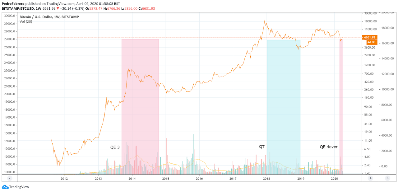Logarithmic chart of Bitcoin from Bitstamp, 2012–2020 (Source: https://www.tradingview.com/x/5xsBmoK5/)

The graph above helps us paint a clear picture of the BTC/USD price performance.

Essentially, it allows us to expand on the idea that investors and traders see bitcoin as a purely speculative asset, almost like forex or stock — which makes sense considering the low volume and liquidity. Even though Bitcoin is seen by hodlers as a hard currency, defined by Investopedia as money that is both issued and seen as politically and economically stable due to low market liquidity, volatility is still quite high.

So far, bitcoin has fallen from a recent high of $10,400 in mid-February 2020 to around $6,800 in late March 2020, according to Bitstamp. That’s a 35% drop in price.

Volume-wise, there has been a significant drop since mid-2019. The trend seems to have stabilized since March 2020, as a few weekly green candles have been popping up.

Still, the cryptocurrency has outperformed most assets, except for precious metals such as gold, a classic SoV commodity.

On one hand, QE seems to positively impact bitcoin’s price. Since bitcoin’s inception, in 2009, there have been two rounds of QE. The first was in November 2010 and the second in September 2012, as we’ve discussed in section two.

Both corresponded with fantastic price appreciation. While during QE 2 BTC/USD increased from less than one dollar to over $40, during QE 3 the price increased from around $10 to over $1000 in early 2014.

On the other hand, QE may be ineffective during shutdowns, since the economy is not producing goods and companies are not spending. Therefore, we could see bitcoin turn bearish, as short-term traders and investors leave the market.

If we look at the QT period, from 2018 to 2019, BTC/USD dropped substantially, from a high of $19,700 to a low of $3,100. In percentage terms, we’re looking at an 85% drop in price, which seems to have been heavily influenced by less liquidity entering the financial markets.

Nonetheless, Bitcoin has maintained a positive price trajectory over the past 10 years, which has been heavily influenced by expansive monetary policies such as QE.

To make our analysis whole, let’s see how gold has evolved during the same period.

The impact of QE on future Bitcoin’s price

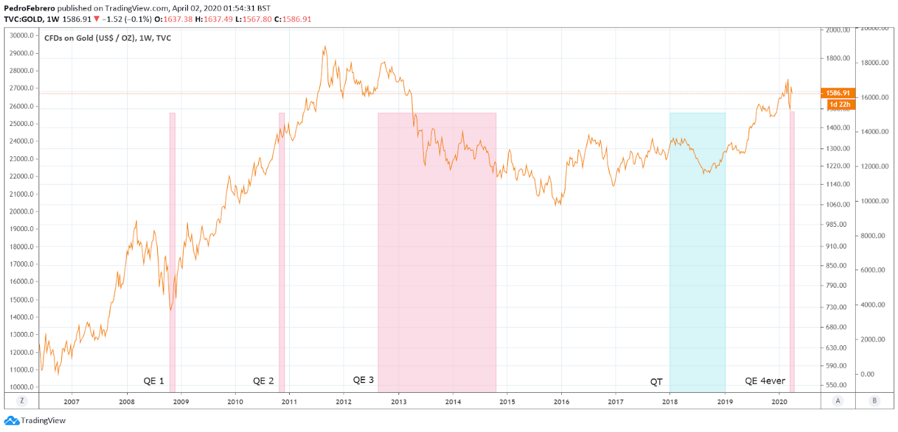This chart shows the price of gold CDFs, 2000–2020 (Source: https://www.tradingview.com/x/l1N9qpbw/)

We will conclude this piece by explaining how QE affects, directly and indirectly, the price of Bitcoin, as well as to hypothesize on the impact of other expansive measures, such as UBI. To do that, we’ll look into the price of gold — which is, theoretically, the most similar asset to BTC in terms of characteristics.

Since QE began, gold has experienced a major bull run, which took its price from just over $700 per ounce, in late October 2008, towards a record high close to $1890 per ounce in mid-August 2011, according to the Tennessee Valley Authority (TVC). Gold’s price increased by 170% between this period.

However, soon after, the price dropped over 20%, and not even QE 3 was able to push it toward another bull run. From October 2012 till early January 2016, gold went from $1770 per ounce to just over $1055, representing a 41% drop in price. It was only after 2016 gold started to pick up the pace again. At the moment of writing, in late March 2020, gold is sitting just over $1620, meaning it increased 53% in price.

The reason why we believe gold took a massive hit was a booming stock market and housing market. Moreover, consumers’ confidence in the Fed to maintain the booming market reached its highest since 2000, in late 2018. Only after QT measures were implemented, gold saw a huge spike in price appreciation, during September 2018.

Nevertheless, QE added enormous liquidity to these markets. The problem now is that the economy has halted and investors are liquidating assets for cash. While the real impact has not been felt on prices, since consumers are quarantined and not spending much, the trend will eventually shift. This brings us to the main driver of hard-money price appreciation.

As additional money floods the economy, through QE, UBI and other expansive monetary policies, consumer confidence will eventually return and inflation will kick in. From the moment consumers return to buying, prices will most likely increase, given the enormous amounts of dollars trapped in the economy.

This sudden drop in the purchasing power of currency could drive up the prices of hard-money assets. Much like what happened to real estate around the world during the past 10 years, where house prices boomed across North America, Europe and Asia, we could now see a similar pattern emerging in the hard-money market.

Because markets are at a period where liquidity is needed, we will most likely see the U.S. dollar remaining king for a while, at least until there is an avalanche of currency flowing into the pockets of consumers.

Hence, every asset or commodity with limited quantities and strong network effects, for example gold, silver and bitcoin, could suddenly increase in purchasing power.

The advantage Bitcoin has over precious metals is that it is extremely fungible, divisible, portable and easy to acquire and exchange. All those traits make it more attractive than traditional commodities.

To conclude our analysis, we would like to emphasize that Bitcoin has two very unique characteristics that make it a harder asset than any other money form in existence. First, we can quickly verify the authenticity of a bitcoin transaction and secondly, it’s fairly straightforward to enforce our right of ownership, by owning our private keys.

Anyone interested in cryptocurrency can open an account with an exchange, purchase bitcoin and withdraw it to a personal wallet or node wallet. Thus, verifying we bought a real bitcoin is fairly straightforward, as a simple transaction will do, and we can quickly enforce our property rights by moving the coins out of the exchange.

This means that the barriers to entry are fewer than in other markets, such as in precious metals, and it’s easier to keep our money within our grasp.

Will QE drive up bitcoin’s price in the medium to long-term?

At the end of the day, it depends on how traders and investors view the Bitcoin network. If most believe it is a safe haven asset, then QE will eventually push up BTC’s price. As currency becomes extremely abundant, assets with strong network effects and limited quantities tend to rise in price.

If the pendulum of monetary policies swings toward hard money during the next few years, BTC could become a monetary reserve, alongside gold and other precious metals.

Safe trades.

---

This article was written by Pedro Febrero, with primary co-editing done by Mati Greenspan, founder and CEO at Quantum Economics, and Charles Bovaird, senior contributor for Forbes and vice president of content at Quantum Economics.

---

Subscribe to WORDS

* indicates required

Email Address *

First Name or Nym *