Debunking Bitcoin’s natural long-term power-law corridor of growth
| If you find WORDS helpful, Bitcoin donations are unnecessary but appreciated. Our goal is to spread and preserve Bitcoin writings for future generations. Read more. | Make a Donation |
Debunking Bitcoin’s natural long-term power-law corridor of growth
By Marcel Burger
Posted November 30, 2019
Some models are useful, some fail to meet required underlying assumptions.
What’s this all about?
After PlanB wrote his (by now) famous piece on the relation between Bitcoin’s stock-to-flow ratio, a lot of people tried to debunk his model, including the author of this piece. It also inspired a lot of people to develop a competing model. But to my knowledge until today no-one succeeded in either a successful academically valid rejection of the model, or to come with a better model. One person in particular keeps coming back saying his model does a better job. Harold Christopher Burger’s idea was to build a comparable model, but instead of taking the natural logarithm of the stock to flow ratio as an independent variable, he thought the natural logarithm of time would be a better input. He reasoned that stock-to-flow is a function of time, so time itself must perform better. Even though Nick has demonstrated repeatedly (here for instance) how PlanB’s model is just better, Harold keeps claiming his work is superior. Time to take a closer look at his model and either applaud him for doing a fantastic job, or just send it (=his model) to the graveyard where it can take a rest with other failed attempts.
Regression again
Just like PlanB’s work, Harold’s work is also based on Ordinary Least Squares Regression. So, we check to see whether all the required assumptions are met. I have mentioned those assumptions as well in the first piece in which I reviewed PlanB’s model. Here they are listed once more.
(1) The expected value of the error term is zero (which means that on average the regression should be correct)
(2) The error and the independent variables should be independent.
(3) The error term should be homoskedastic (i.e. error terms have the same variance)
(4) There should be zero correlation between different error terms (i.e. autocorrelation is excluded)
After checking whether these hold, I’ll also take a look if cointegration applies here even though cointegration with time doesn’t make much sense. I’ll follow the same procedure as followed when reviewing PlanB’s work.
Data and Model
To build the model I used the CoinMetrics dataset which can be found here. All data before a price tag for bitcoin was known is discarded. The first day of the dataset is presented as day 1, the second day as day 2 and so on. So we’re counting the days as of day the first price tag is available. We take natural logarithms of both the price tags and the day counts. So our data starts like this:
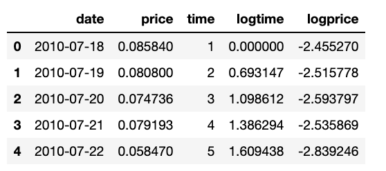 Start of the dataset with time as days counted since start of the set
or like this:
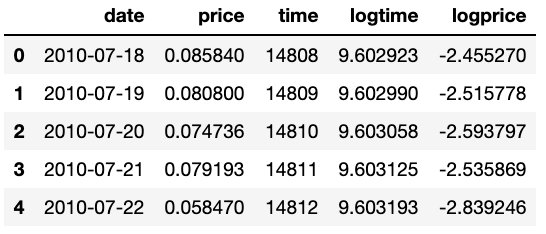 Start of the dataset with time as days counted since Jan 1st 1970 (UNIX)
or like this:
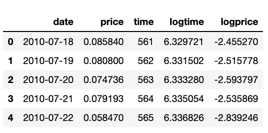 Start of the dataset with time as days counted since bitcoin’s Genesis block (Jan 3rd 2009)
Building the model and testing assumptions
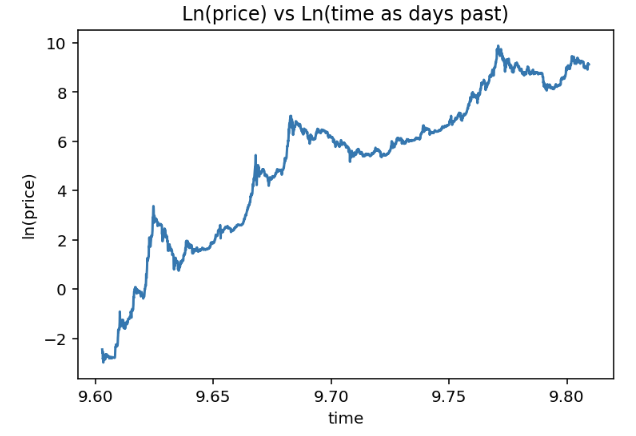
Before we start checking whether the assumptions hold up, we’ll start with some visual inspections of the data. Let’s see how the log-log chart looks like in case we work with time as days past since first measure. Time is a relative concept, so the performance of the model will be dependent of the point in time we consider as point 0.
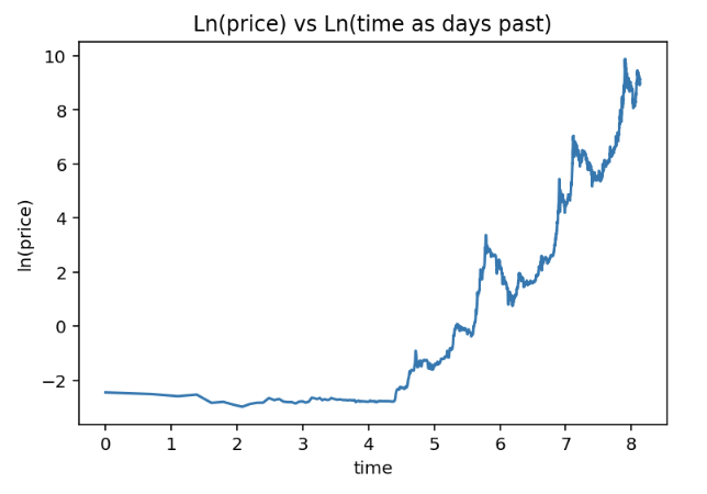 Relation between ln time and ln price as time is days since first available price tag for bitcoin
Another logical starting point would be January 1st 1970 as day 1, we’ll go with that and look how the relation changes.
 Relation between ln time and ln price as time is days since 1–1–1970
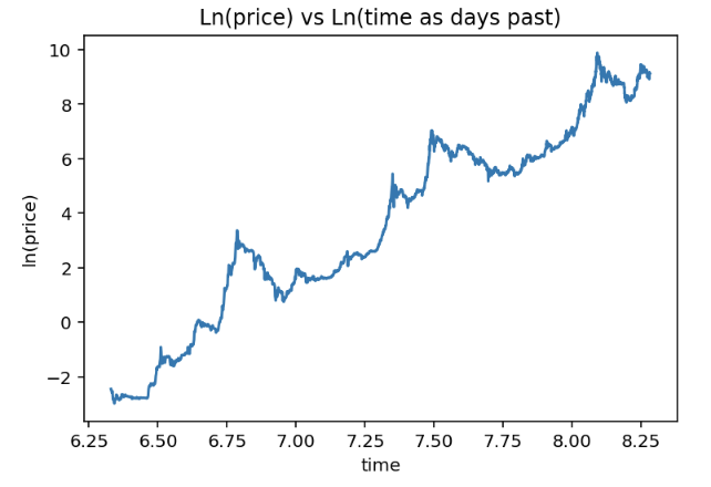 Relation between ln time and ln price as time is days since January 3rd 2009
Starting to count the days as of the 3rd of Jan 2009 while first prices are not available seems a bit strange to me. It feels a bit like cherry picking the most suitable relative time series. This is what Harold used in his model, so we go with it as well here. Taking the first two would not return meaningful results as there would be too much non-linearity in those relations anyway. I would like to remark that this is where the model already starts to become shaky.
After running the regression, it’s time to take a closer look at the regression results and to research the model residuals. Here’s the regression result:
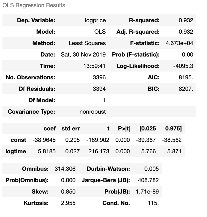 Regression results for ln time vs ln price
Even though R-squared is quite high, R-squared is not a very meaningful metric when we evaluate the regression of two non-stationary time series. It often turns out to be quite high when we’re using trending series and we should be aware of spurious regression. Further, the coefficients seem to be both significant, but the main question is whether the underlying model assumptions are met.
Residual analysis
We’ll take a look at the residuals to check for possible issues with the model.
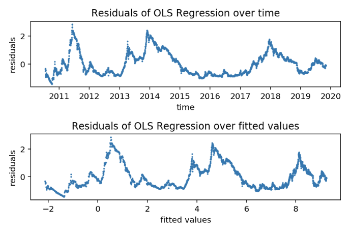 Plots of the residuals that follow from the regression
There’s a very clear pattern observable in both plots, which tells us that the residuals are likely to be autocorrelated, which would mean that the 4th assumption is not met. Next to that, we can also clearly see that the variance differs over time, which would indicate that the 3th assumption is violated as well. Both violations would lead to a falsification of the model.
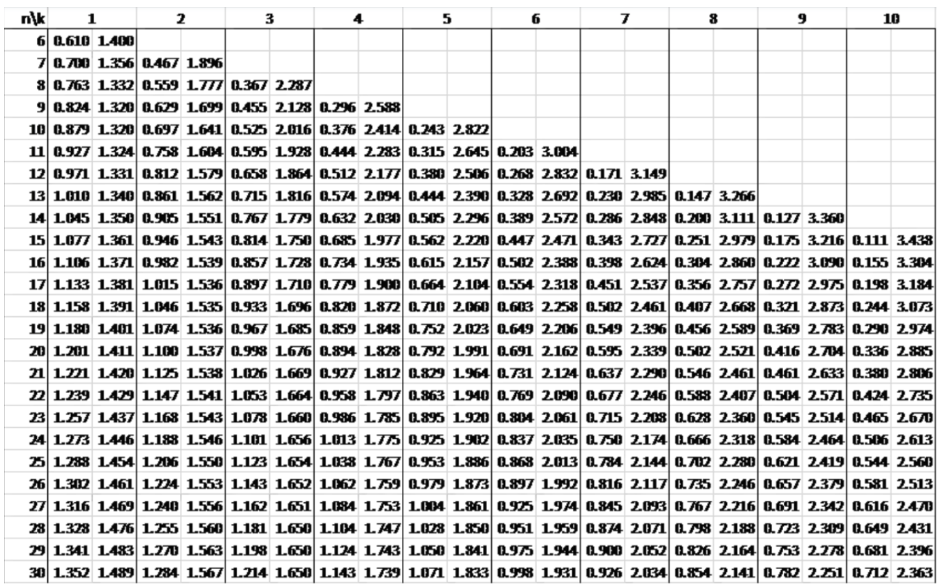
We will test for autocorrelation to make sure that this is an issue. The Durbin Watson statistic turns out to be 0.005 (check OLS results above) which is much smaller than the allowed lower bound value (see DW table in the Appendix).
Sofar, I would conclude the model’s fundamentals are no good, and the only reason to not reject it, would be in case we can show the variables are cointegrated.
Cointegration and Order of Integration
In order for two time series to be possibly cointegrated, those time series have to be integrated of the same order. Time to check how the both series are integrated, as they are both clearly non-stationary (both series trend up). Let’s have a look at the original series and their first differenced series. (Differencing means taking the difference of two consecutive values in the same time series.)
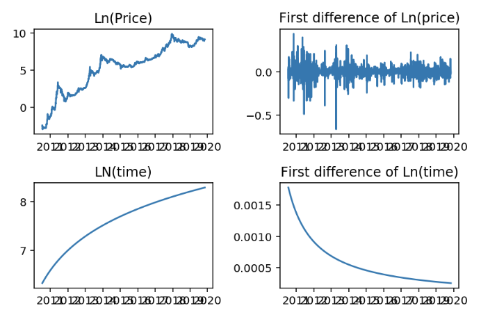 Variables over time and their first differenced series
The charts above show that both time series are not stationary. Ln(price) is integrated of the first order as it shows to be stationary after differencing the series once. For log(time) we have to look further, as differencing once didn’t result in a stationary series. We keep on differencing to find the integration order for log(time), which resulted in the following:
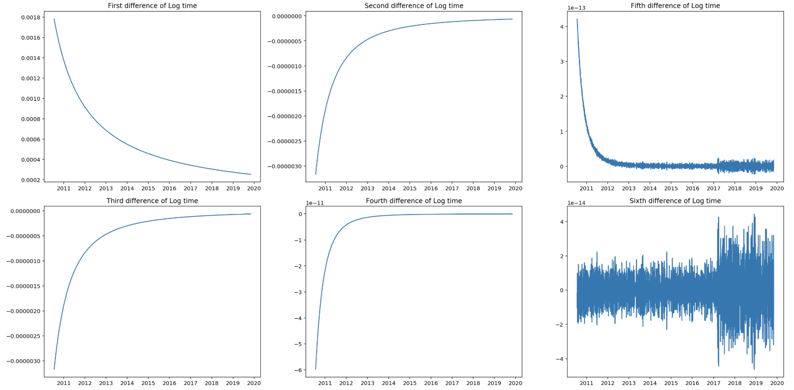 Log(time) seems to be 6th order integrated.
Log(time) seems to be integrated of the 6ht order. This tells us that both variables are integrated of a different order and therefore cointegration is off the table. No need to run any further checks or statistical tests, as this requirement is not met.
EDIT: The 6th order integration as mentioned above is not proven by any test. In fact I learned that it even might not be reaching stationarity at all. The graph showing the sixth order difference, illustrates that we reach the limitations of the computer, as we witness floating point noise. For the conclusion it doesn’t matter. Special thanks to Hmatejx for pointing this out.
Conclusion
The model as developed by Harold Christopher Burger (more detail here: https://medium.com/coinmonks/bitcoins-natural-long-term-power-law-corridor-of-growth-649d0e9b3c94) is falsified. Since the model is falsified there is no need to compare it to any other model and PlanB’s stock to flow model in particular. A first threshold to compare a model to other models is that it should meet the fundamental assumptions.
Appendix
Durbin Watson table
References
- https://medium.com/@100trillionUSD/modeling-bitcoins-value-with-scarcity-91fa0fc03e25
- https://medium.com/coinmonks/bitcoins-natural-long-term-power-law-corridor-of-growth-649d0e9b3c94
- CoinMetrics Datasets, https://coinmetrics.io/data-downloads/
- M. Verbeek, A Guide To Modern Econometrics
- http://www.real-statistics.com/statistics-tables/durbin-watson-table/