Bitcoin’s increasing price resistance uphill, short and long-term

If you find WORDS helpful, Bitcoin donations are unnecessary but appreciated. Our goal is to spread and preserve Bitcoin writings for future generations. Read more.

Make a Donation

---

Bitcoin’s increasing price resistance uphill, short- and long-term

By Harold Christopher Burger

Posted December 30, 2019

What can we say about bitcoin’s future price? In “Bitcoin’s natural long-term power-law corridor of growth” I have proposed a mathematical model for bitcoin’s price evolution which uses a simple equation using only time as an input variable. This article will not use a precise mathematical model. Rather, we will make a number of empirical observations regarding bitcoin’s price evolution. Two main observations are made:

• The case for the fact that bitcoin’s price returns are diminishing over time (i.e. price growth is slowing) is strengthened.
• Bitcoin’s shorter-term price movements are becoming tamer over time: Fluctuations are becoming less extreme in the short-term.

These two points can be explained by the fact that it takes more and more capital to increase the price of bitcoin, and that it becomes more and more difficult to find more capital. Moving the price of bitcoin from $0.1 to $1 was possible with relatively few dollars. Moving the price of bitcoin from $1000 to $10000 required much more capital. This effect slows the potential growth of bitcoin in both the long- and short-term.

The price of bitcoin is facing more and more resistance on its path upwards. To a lesser extent, the same is true for downward price movements.

Investors should expect lower long-term gains than in the past, but also tamer and slower bull markets. Overall, bitcoin’s price volatility indeed seems to decrease with time. Price growth here should be understood as being in percentage terms.

The red zones are reflections of the statistics of short-term growth rates observed within the halving period. The highest and lowest points in the reddish areas represent the maximum and minimum growth rates observed. The maximum and minimum growth rates are estimated over several hodling periods, represented horizontally. Darker areas indicate percentiles. The exact process is described further below in this article.

Diminishing or non-diminishing returns?

Bitcoin’s price history is best looked at by using a logarithmic scale for the price, giving us as so-called semi-log plot, in which the x-axis represents time and is linear, and the y-axis displays the price of bitcoin, and is scaled logarithmically.

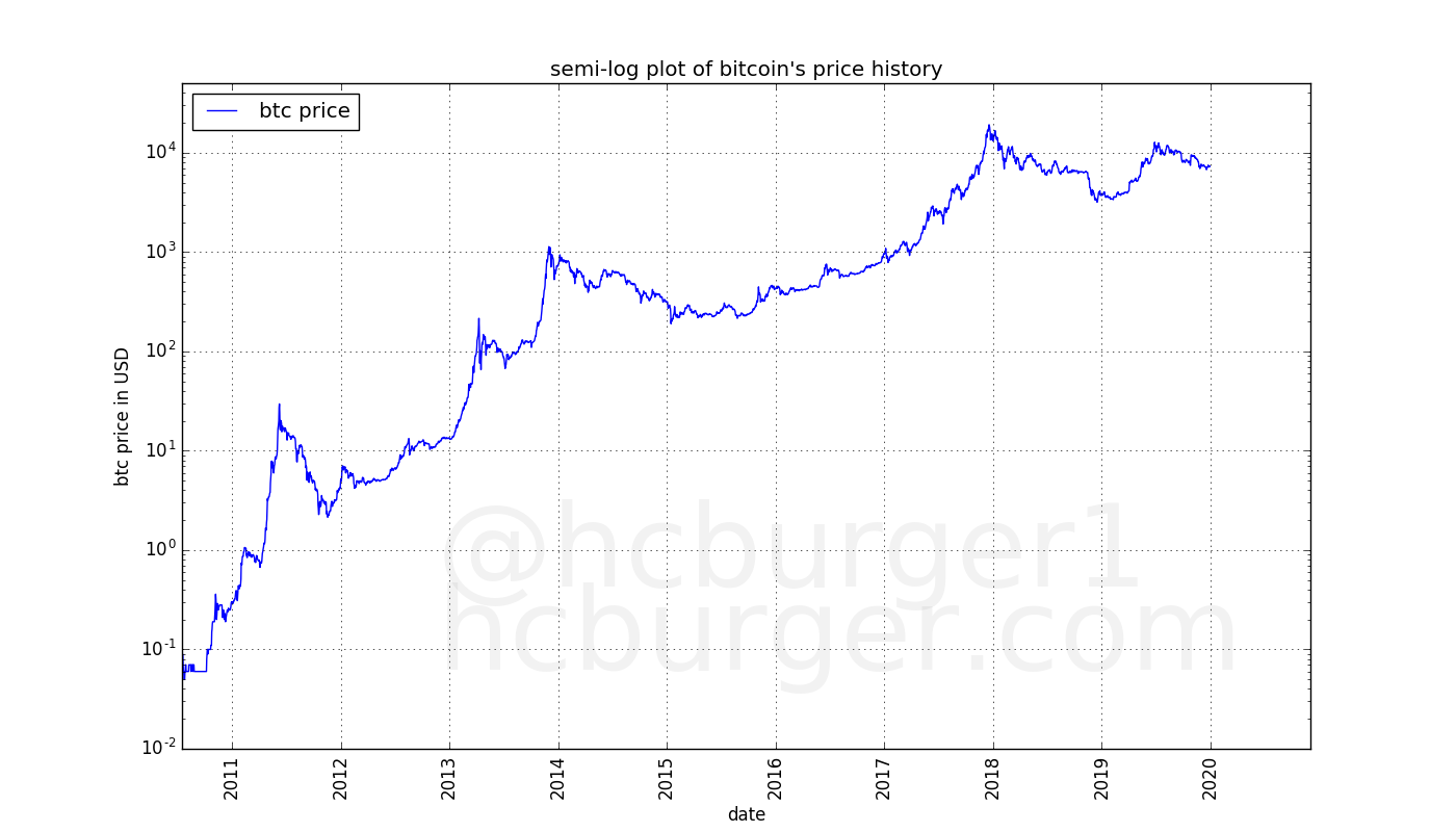
Using a logarithmic scale gives us the advantage of being able to observe bitcoin’s full price history in a single plot. It also has the property that equi-distant movements on the y-axis indicate price changes that are identical in percentage terms. E.g. the price movement from $1 to $10 per bitcoin takes up the same distance on the y-scale as the price movement from $100 to $1000. This property is extremely useful but is not always perfectly understood.

To better understand the properties of a semi-log plot, let’s look at two models:

• one with non-diminishing returns (equal expected growth rates over time)
• one with diminishing returns (growth rates become smaller over time)

I used the equation described in the previous article for the model with diminishing returns, but a different model with slowing growth rates could have been used as well for the purposes of this article.

The model with non-diminishing returns displays like a straight line in the semi-log plot, whereas the model with diminishing returns displays like a curve that initially grows quickly, and then more slowly.

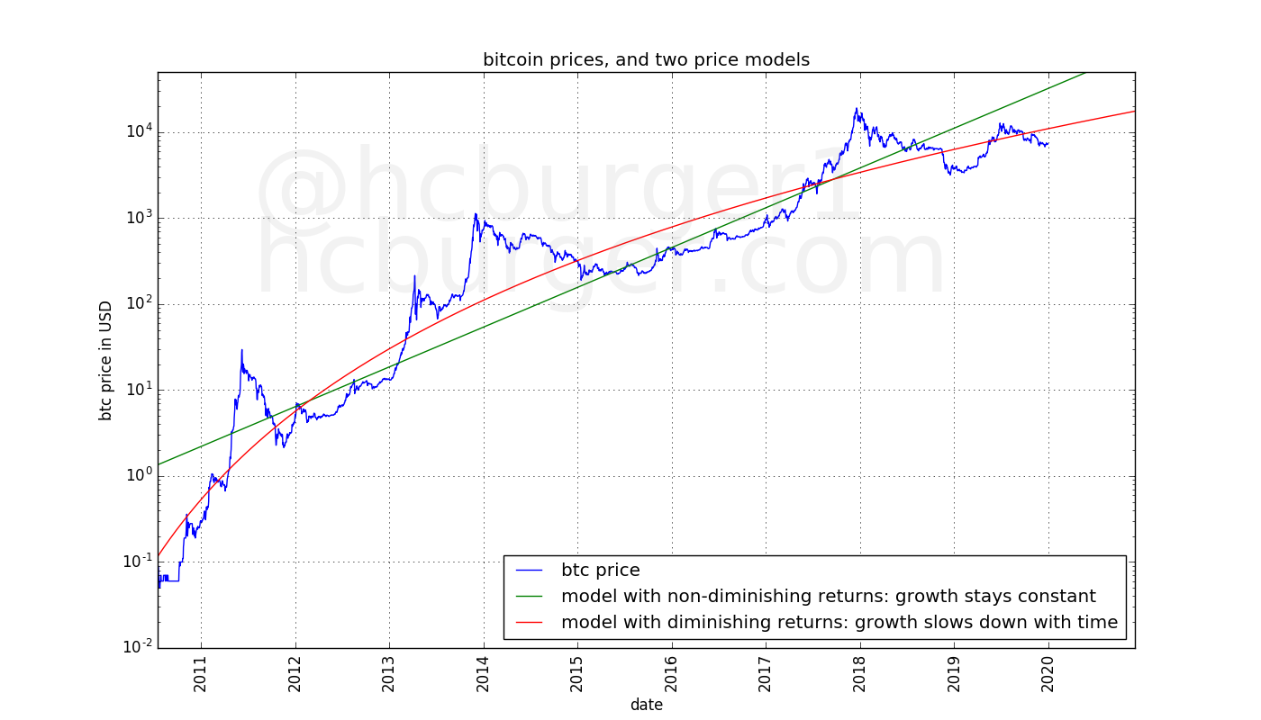
Which model should we prefer? The difference between the two is important, as the two predict wildly different prices in the future.

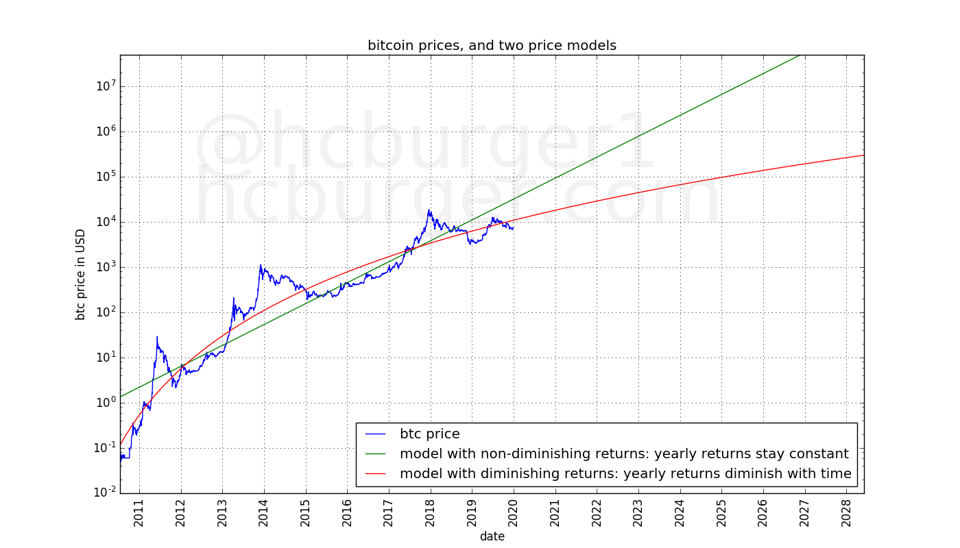
In the previous article, the choice for a model with diminishing returns was mostly motivated by the fact that the bitcoin price curve in the semi-log plot appears to be slowing. Also, the regression error for the model with diminishing returns is “good”: It is about 5.3 times lower than for the model with non-diminishing returns. The model with diminishing returns is therefore empirically better at modeling the data. This already tells us that bitcoin’s long-term growth has diminishing returns, but in this article, we will make some observations that give additional weight to the conclusion that bitcoin’s upward price movements face greater and greater resistance.

Expected returns, long term

Diminishing returns means that bitcoin’s growth is slowing. Non-diminishing returns means that bitcoin’s growth is not slowing down, i.e. the expected growth rate stays the same over time. To better understand the difference between the two, let’s take the perspective of fictional investors.

A model with non-diminishing returns

Let’s assume that bitcoin’s price follows a non-diminishing model. How much money can an investor expect to make? The answer depends on the amount of time the investor held his bitcoin before selling them (the “hodling period”). The longer the hodling period, the higher the expected return. What is interesting is that for the model with non-diminishing returns, the profit the investor can expect to make does not depend on when he invested.

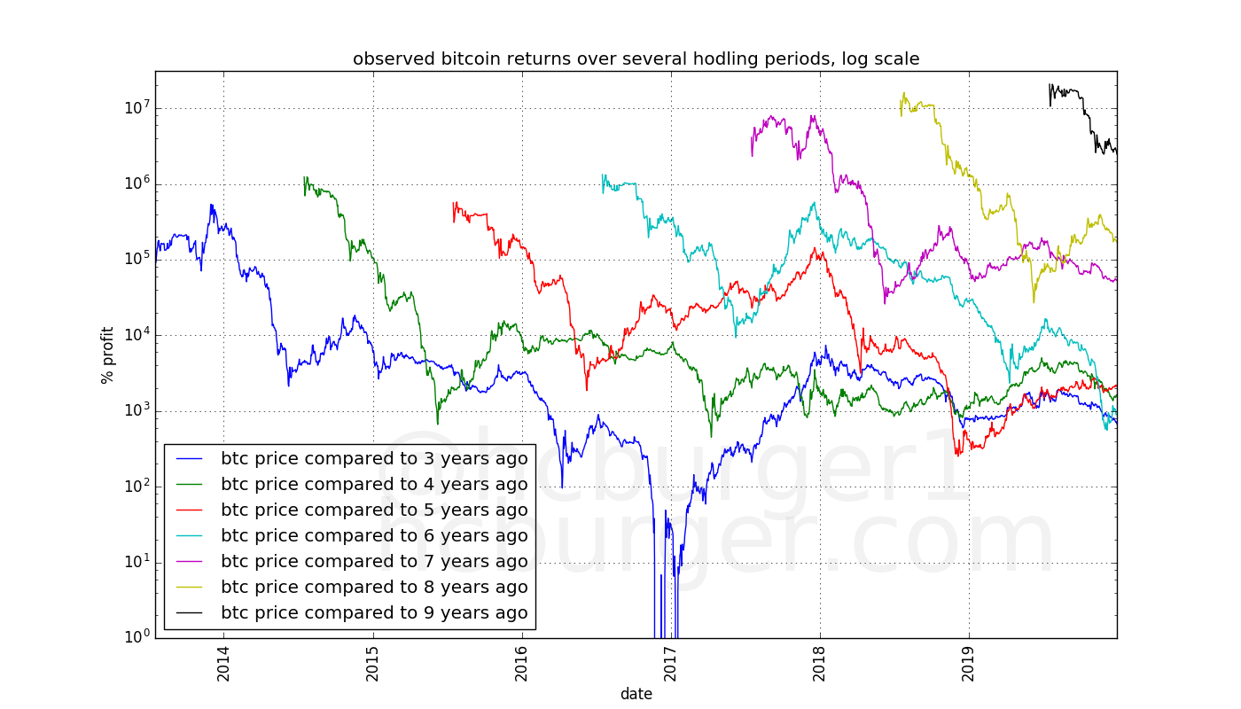
This is demonstrated in the plot below. Each colored line represents one hodling period. The x-value of each point on the line represents the time at which the investor sold his bitcoin. The y-value represents the percent profit he made from his investment.

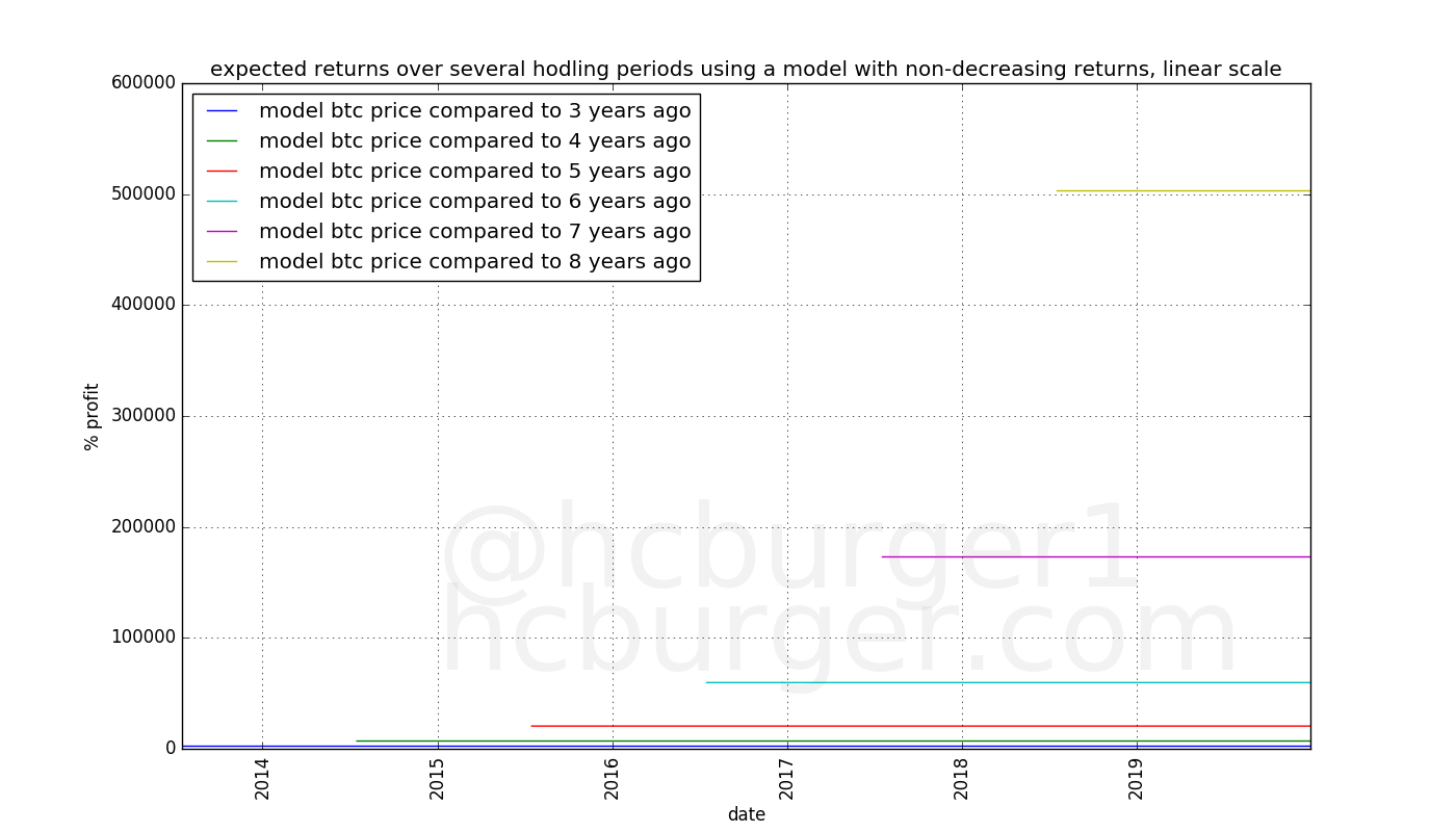
The longer the hodling period, the later the starting point of the line representing that hodling period. This is because bitcoin’s price history is limited and we assume that it was not possible to invest in bitcoin before the 17th of July 2010. According to this, it is not possible to have held bitcoin for eight years before mid-2018, which is why the yellow line above starts in mid-2018.

We can display the same data in a semi-log plot:

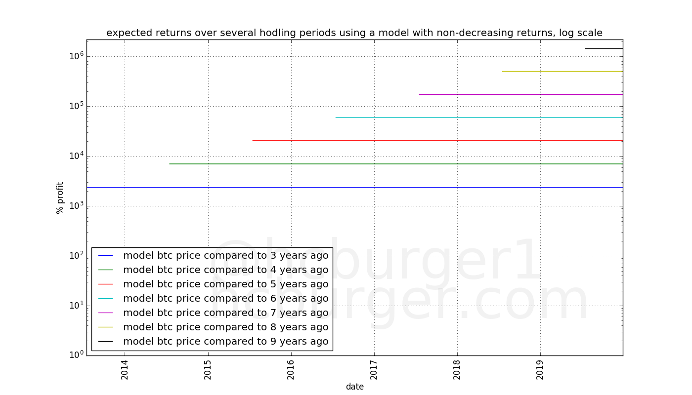
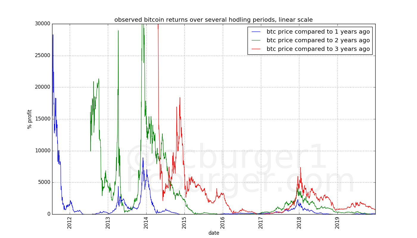
We see that according to this model, an investor who bought bitcoin and sold them 3 years later would have made a profit of approximately 2500% no matter when this investor bought his bitcoin. The same holds true for any other hodling period, but the returns are higher for longer hodling periods.

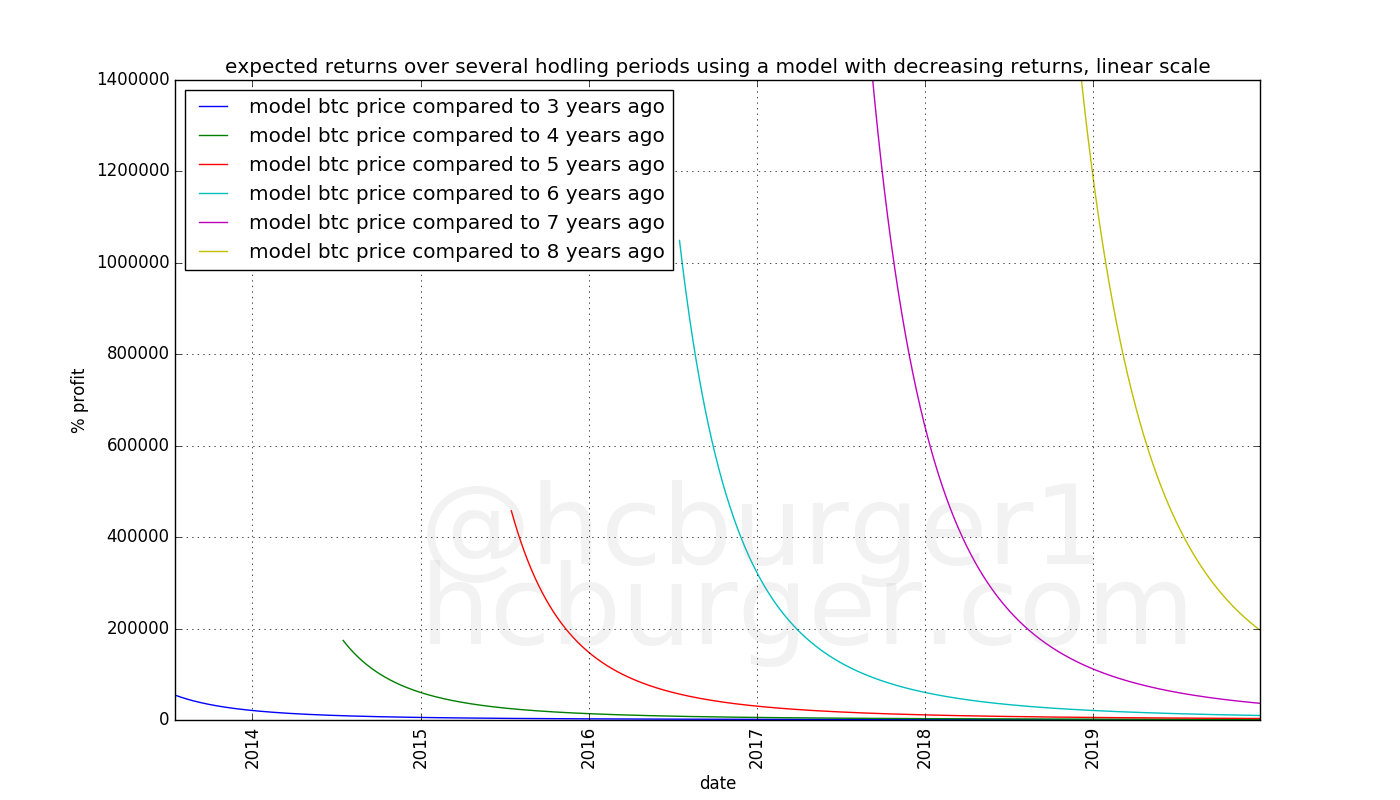
A model with diminishing returns

Using a model with diminishing returns, the situation is different: The expected returns depends on when one invested. The lines in the below plot drop sharply, which means that for the same hodling period, buying earlier gives higher expected returns.

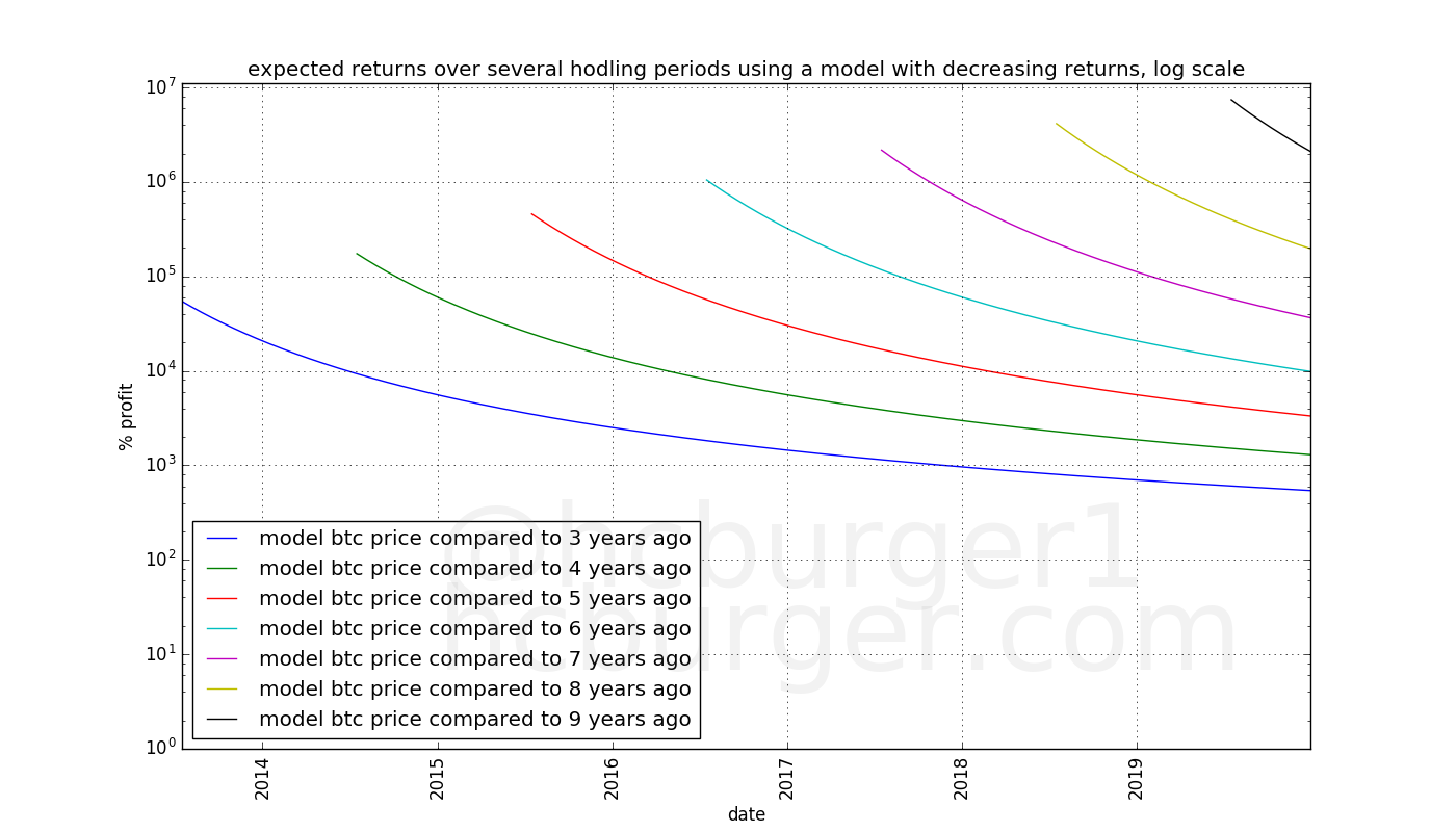
A semi-log plot again makes the data easier to read:

Investor A who bought bitcoin in mid-2011 and sold them three years later in mid-2014 would have made about 10000% profit.

Investor B who bought bitcoin in January 2015 and sold them three years later in January 2018 would have made “only” about 1000% profit, or 10 times less than investor A.

The situation is similar, but even more pronounced for longer hodling periods. A 10x decline in returns occurs faster. Investors A and B invested three and a half years apart, with a 10x difference in returns. For an 8-year hodling period, a 10x decline in returns occurs in about a year.

(Note: For the model with diminishing returns, I used the same model as in my previous article , but the exact choice of the model is not very important here, as the specific numbers are not as interesting as the principle itself.)

Actual returns

The profiles of the expected returns are very different for the model with diminishing compared to the model with non-diminishing returns. The difference is extremely important to anyone who invests in bitcoin. Which of the two models better reflects reality?

To answer this question, we will perform the same exercise as before, but using bitcoin’s actual price history:

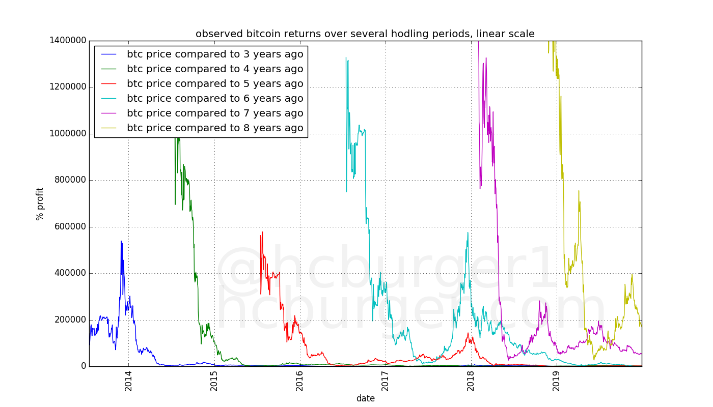
What is immediately noticeable are sharp drops in the return curves, which is in agreement with the model with diminishing returns. What is also immediately noticeable is that the curves are much more noisy than those based on model (i.e. simulated) data. The noisiness is due to the wild price swings for which bitcoin is so famous.

In the semi-log chart, we notice very low returns for the 3-year hodlers around the 2017 mark. This is because the price around 2017 was about $1000, approximately the same as during the previous all-time-high, around 2014. Someone who bought at that all-time-high and sold three years later could have made a small loss.

Let us now compare the real return curves to those based on model data using a model with diminishing returns. The same color-code is used for the length of the hodling periods:

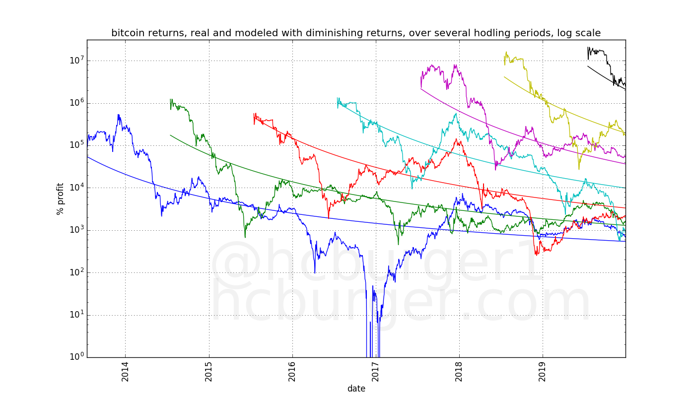
We see that the real return curves are modeled adequately by the model with diminishing returns, but we have to take into account that there is quite a lot of noise.

We can also repeat the experiment for shorter hodling periods, and see a similar, but more noisy, pattern.

The return curves above show us that by the end of the year 2014 at the latest, the nature of bitcoin’s diminishing returns should have become apparent. Later data confirmed that trend.

Conclusions regarding long-term trends

The return curves empirically favor a bitcoin price model with returns that diminish over time. Looking at the three- and four-year return curves, this effect would have been observed at the latest by the end of the year 2014. Newer data has only been confirming this conclusion.

The effects of diminishing returns, combined with price volatility, are:

• The expected returns for all hodlers diminish over time
• The expected returns for long-term hodlers become closer to those of shorter-term hodlers. Due to price volatility, this also means that short-term holders can sometimes have higher returns than long-term hodlers.

The conclusions regarding long-term diminishing returns were already drawn in “Bitcoin’s natural long-term power-law corridor of growth” but we have looked at this effect in a novel way in this article, and have also seen that the effect would have been visible as early as 2014, or maybe even earlier. Also different from the previous article is that we arrive to similar conclusions without using a precise model. The general conclusions are therefore independent of the exact choice of the model.

Why is the price growing slower and slower?

Given the observation that bitcoin’s price growth exhibits diminishing returns, can we come up with a plausible ad-hoc explanation?

Probably the simplest explanation is that increasing the price of bitcoin by a certain amount in percentage terms requires more and more fiat currency. To illustrate: Increasing the price of bitcoin by 100% took relatively little capital when the price of bitcoin was $0.1. It requires much more capital to move the price of bitcoin from e.g. $10000 to $20000.

Attracting ever more capital becomes ever more difficult, or at least, takes more and more time. Perhaps a single individual with modest funds could have moved the price from $0.1 to $0.2, but it would take a very wealthy individual to move the price from $10000 to $20000. Alternatively, the price could be moved from $10000 to $20000 by a greater number of individuals.

Attracting more and more people to invest in bitcoin, or finding a few exceptionally wealthy individuals takes more and more time.

Short-term price changes

Does the above explanation for slower long-term growth rates also have an effect on shorter-term growth rates? This is something that has not been thoroughly considered in “Bitcoin’s natural long-term power-law corridor of growth”. Yet, higher bitcoin prices should make it more difficult to move the price in the short-term, too. This would mean that short-term price swings should become more tame over time, leading both to overall lower volatility and also potentially slower bull markets.

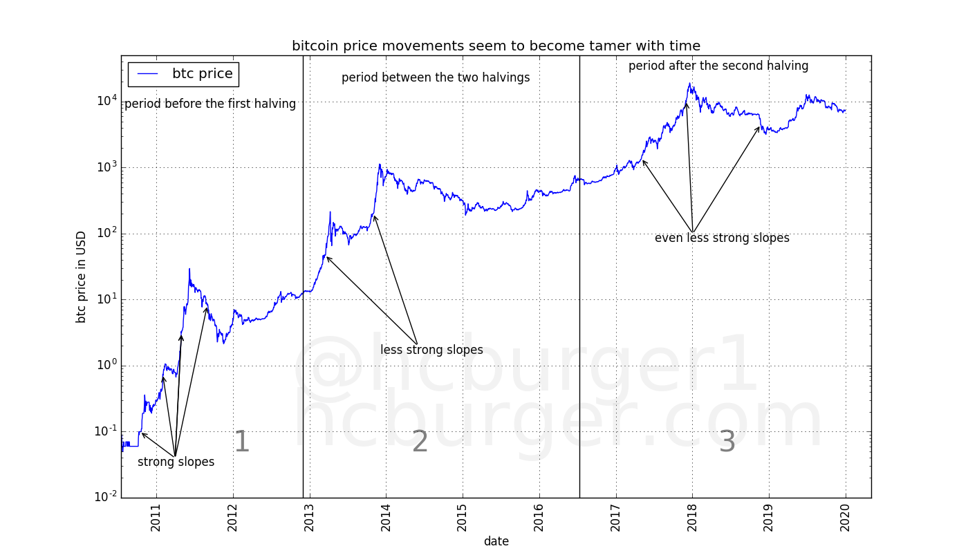
To answer this question, let’s divide bitcoin’s price history into three parts, one for each halving period:

• the period before the first halving (“halving period 1”),
• the period after the first halving and before the second halving (“halving period 2”), and
• the period after the second halving (“halving period 3”).

We observe the strongest price swings during bitcoin’s bull markets. The corrections following a bull market also have strong (downward) price swings. At first sight, it would appear that these shorter-term price movements become slower in the later periods, which also leads to bull markets taking longer and longer to develop:

Let’s consider the slopes of the price curve. A given slope corresponds to a given price change in percentage terms, due to the nature of semi-log plots. Instead of talking about price changes in percentage terms, we can talk about differences in the log price. The two are completely equivalent.

In each period, let’s consider the slopes of bitcoin’s price movement over a particular timeframe, e.g. 180 days. For each 180 day timeframe, we will look at the difference between the log price at the beginning and the log price at the end of that timeframe. We then count how often this difference falls into a particular range. The result is a histogram of bitcoin log price growth rates over 180 days. The growth rates are equivalent to slopes in the semi-log plot of the price history. Negative log price changes mean that the price has been declining.

The histogram of the 180 day growth rates for the three halving periods can be displayed in a table:

(Period 1 corresponds to the period before the first having, period 2 to the period between the two halvings, and period 3 to the period after the second halving).

What becomes immediately apparent is that the earlier halving periods have more extreme growth rates, in both the positive and negative direction. For example, the first period had 180-day growth rates of between -1.01 and -0.57 and also between 1.08 and 2.18, whereas the later halving periods do not. The second halving period has 24 instances of 180-day growth rates of between 0.97 and 1.08, whereas the third has none.

The same data can be displayed visually, allowing for easier inspection:

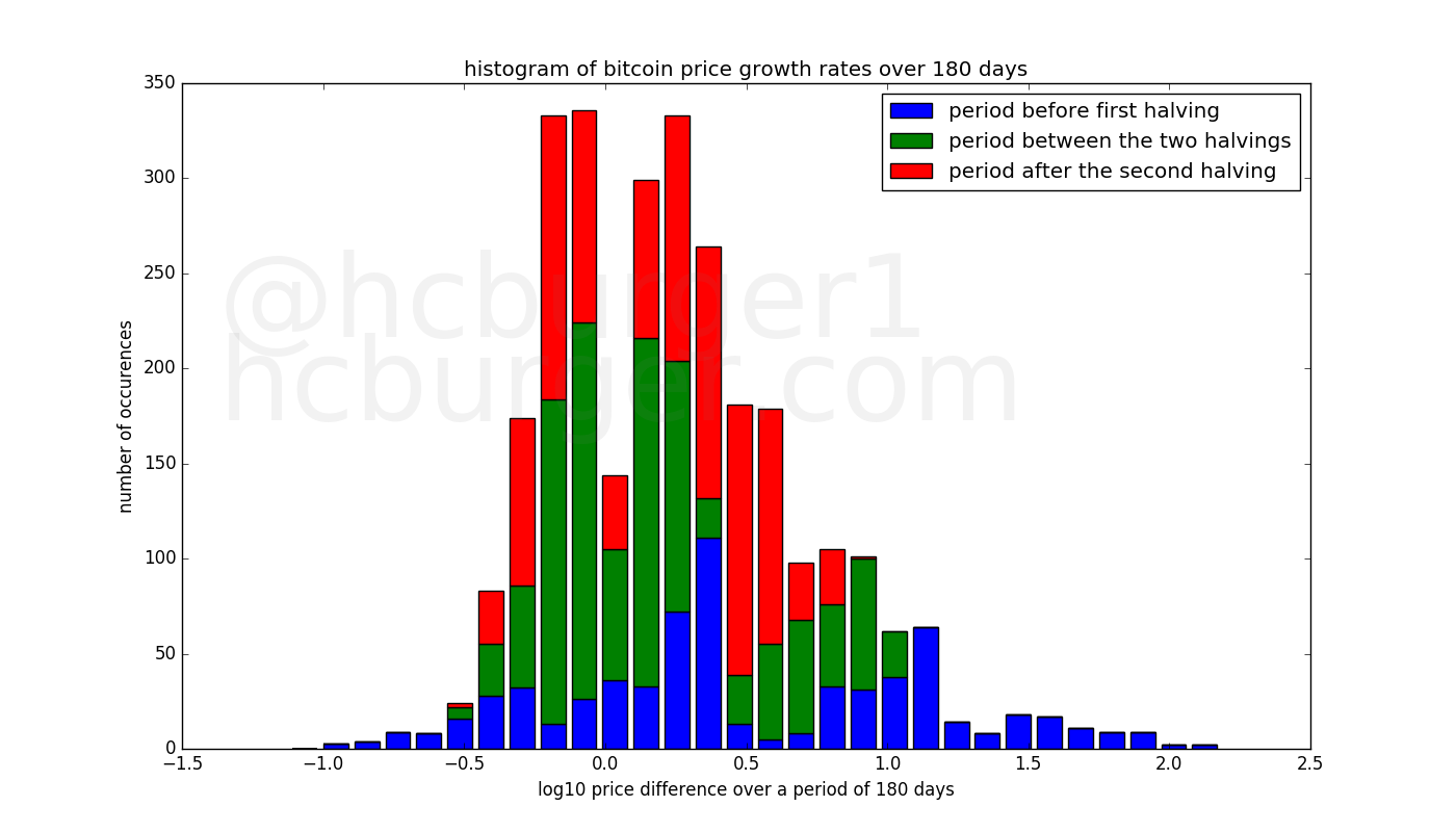
The blue bars representing the distribution of the growth rates of the first halving period are more spread out than the green and red bars representing the two other periods. A greater vertical size of a bar indicates a higher count in that bin. The earliest halving period is the most spread out, the second less so, and the third halving period the least.

Alternatively to the histogram, we can also consider the statistics of the 180-day growth rates for the three periods. The first number is expressed in log10 terms, whereas the number in parenthesis is expressed in percentage terms.

Halving period 1 (before the first halving):

• max growth rate: 2.156613 (14242 %)
• 90th percentile growth rate: 1.410404 (2473 %)
• 10th percentile growth rate: -0.352216 (-56 %)
• min growth rate: -0.996782 (-90 %)

Halving period 2 (between the two halvings):

• max growth rate: 1.079093 (1100 %)
• 90th percentile growth rate: 0.810624 (547 %)
• 10th percentile growth rate: -0.225461 (-40 %)
• min growth rate: -0.518089 (-70 %)

Halving period 3 (after the second halving):

• max growth rate: 0.862816 (629 %)
• 90th percentile growth rate: 0.586342 (286 %)
• 10th percentile growth rate: -0.251239 (-44 %)
• min growth rate: -0.465312 (-66 %)

The maximum growth rate over a 180-day hodling period was 14242% in the first halving period, 1100% in the second, and 629% in the third halving period. The strongest negative growth rates over a 180-day hodling period was 90% in the first halving period, 70% in the second, and 66% in the third halving period, indicating that downward swings (over a 180-day span) have also become tamer over time.

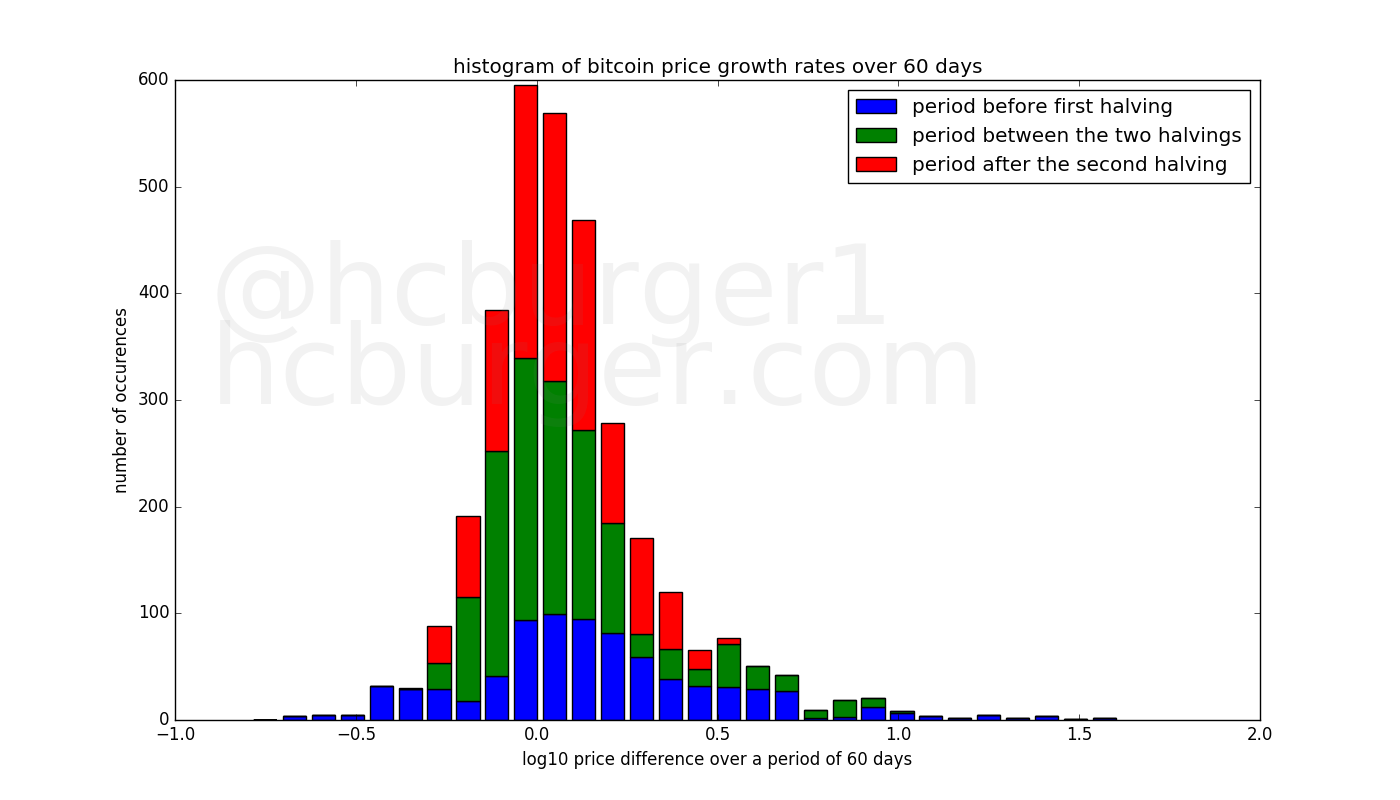
Similar observations can be made when the 180-day holding period is changed, e.g. to 60 days:

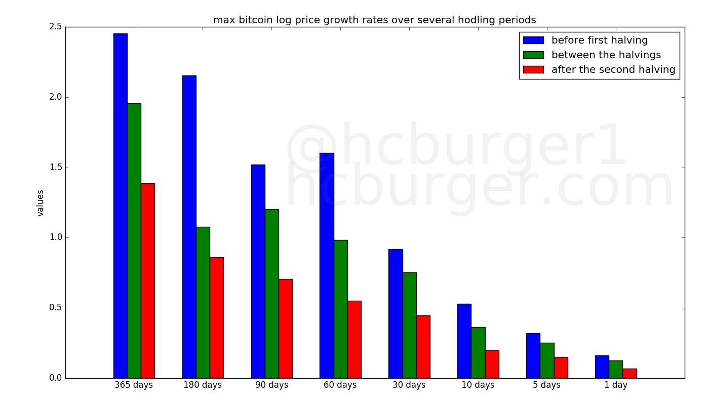
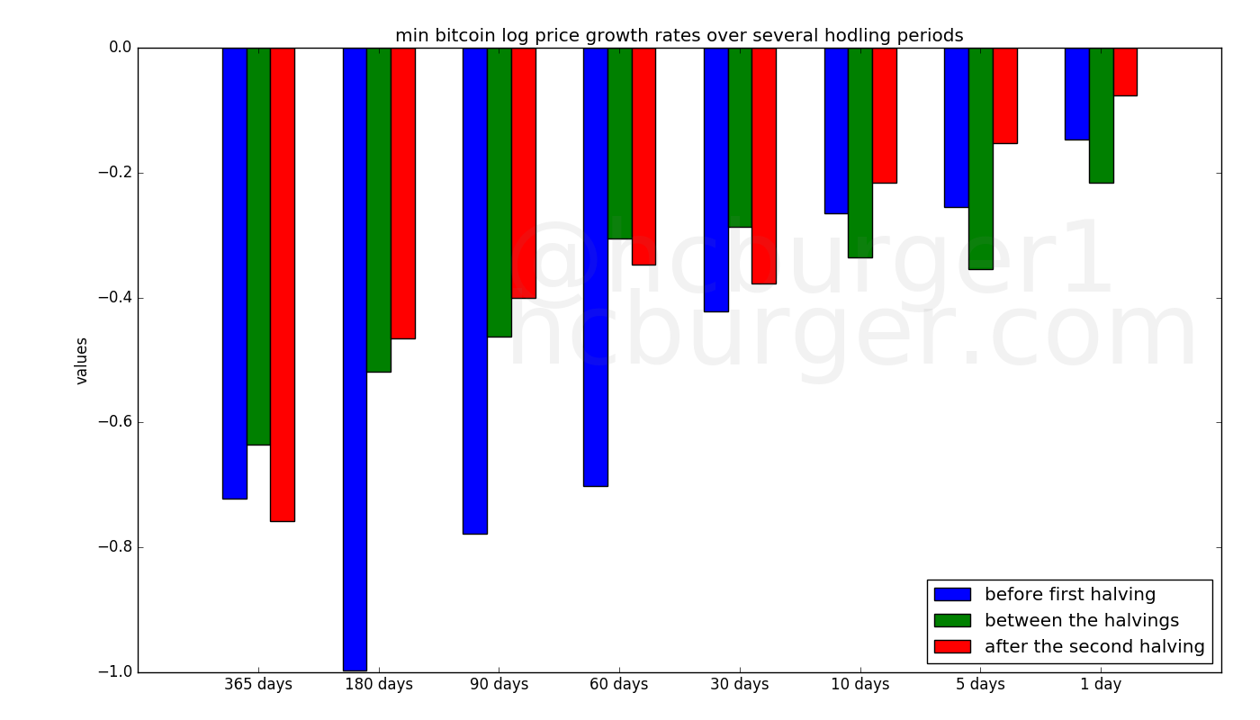
The maximum growth rate over several hodling periods systematically declines over the three bitcoin halving periods:

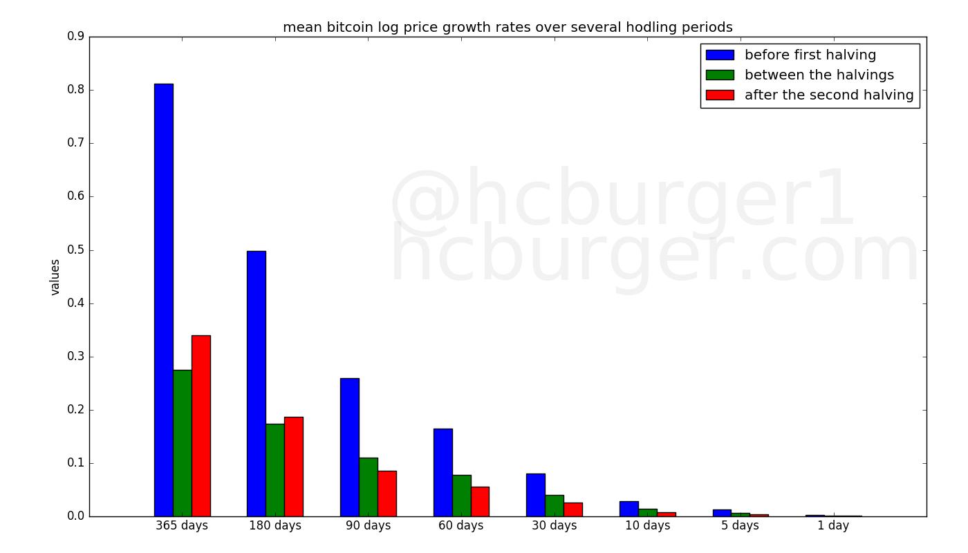
The mean growth rates over most hodling periods also declines over the three halving periods. This is just a reflection of the fact that the price of bitcoin has been increasing at a slower and slower rate.

The value of the minimum growth rate over several hodling periods also tends to decrease over the three halving periods, though this effect is less marked than for the maximum growth rate.

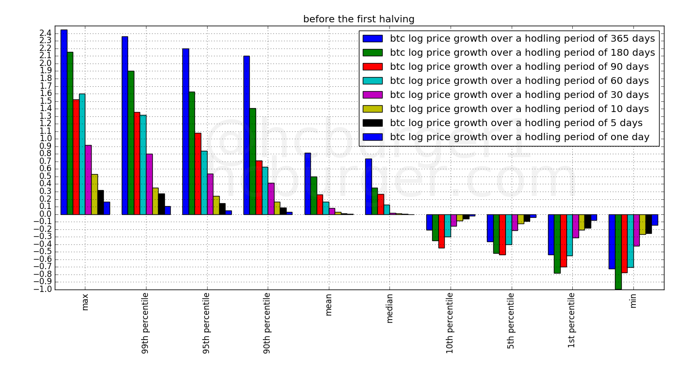
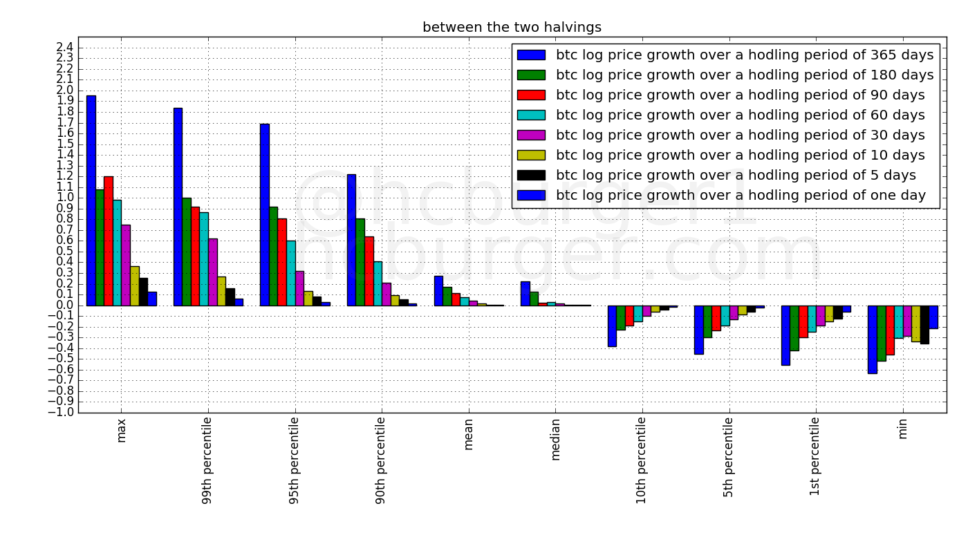
Let’s now make one plot per halving period. Each plot contains several statistics over several hodling periods. The percentiles are statistics that lie between the min and the max, so that e.g. the 90th percentile can be used as a form of “attenuated max”, or the 10th percentile as a form of “attenuated min”. The 50th percentile is the same as the median.

The following plot displays the statistics for the first halving period:

The next plot displays the statistics for the second halving period. The y-axis still uses the same scale. The fact that almost all bars have shorter length means that the statistics over most hodling periods have been attenuated.

The statistics are further attenuated from the second to the third halving period:

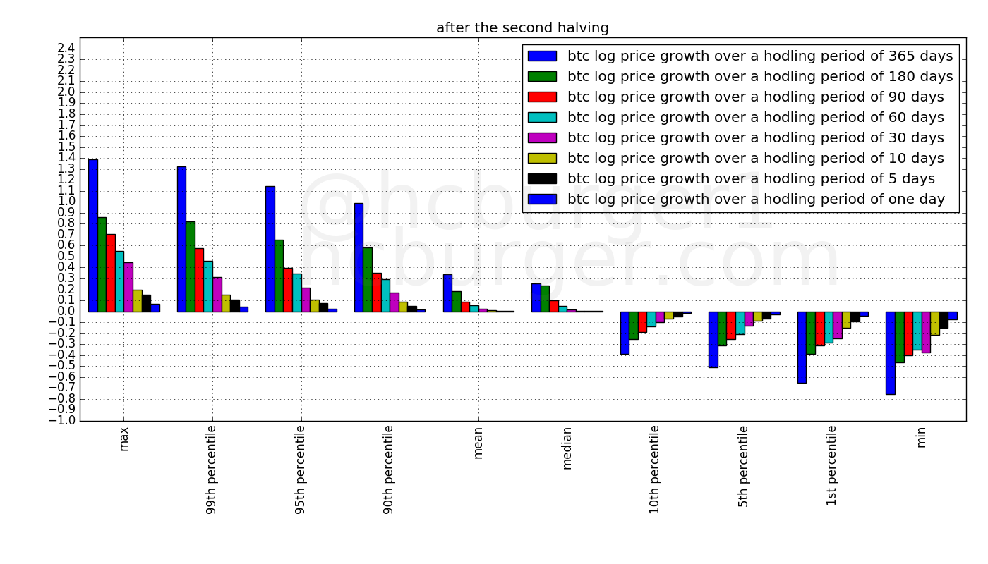
These three plots confirm that the positive growth rates over relatively short hodling periods become smaller and smaller in each succeeding halving period. To a lesser extent, negative growth rates also become smaller over time.

These observations are in agreement with our explanation that it takes ever more capital to cause price fluctuations, and hence price fluctuations become tamer. We should expect this trend to continue in the future.

The statistics computed above can also be represented graphically. In the following plot, we display the statistics of each halving period at the end of that halving period, anchored at the price at that given time. The vertical width of the red regions represents the difference between the min and the max growth rates. The red regions have a horizontal width of 365 days because that is the longest short-term hodling period we have considered. Darker red tones just represent different percentiles.

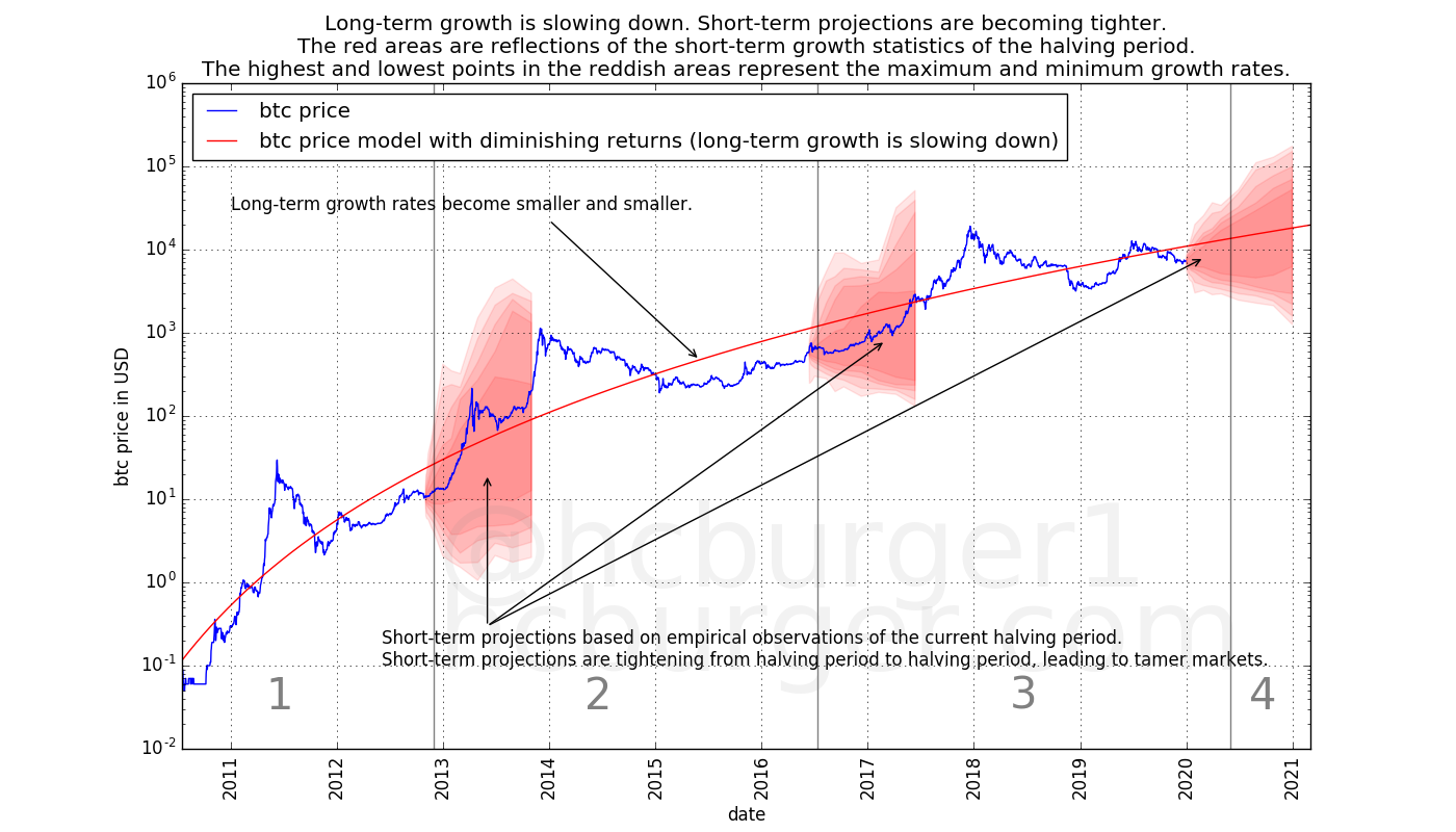
This is another convenient representation showing that the statistics over the short term have become tamer in successive halving periods.

Future price developments

We have two ways of looking at price predictions and models. Assessing whether:

• the long-term projections are realistic
• the short-term projections are realistic.

Let’s look at a few potential scenarios.

Predictions made by individuals

It appears that it is believed by some that bitcoin’s price will grow with non-diminishing returns, leading to some price predictions being made that are more in-line with the model with non-diminishing returns than with the model with diminishing returns:

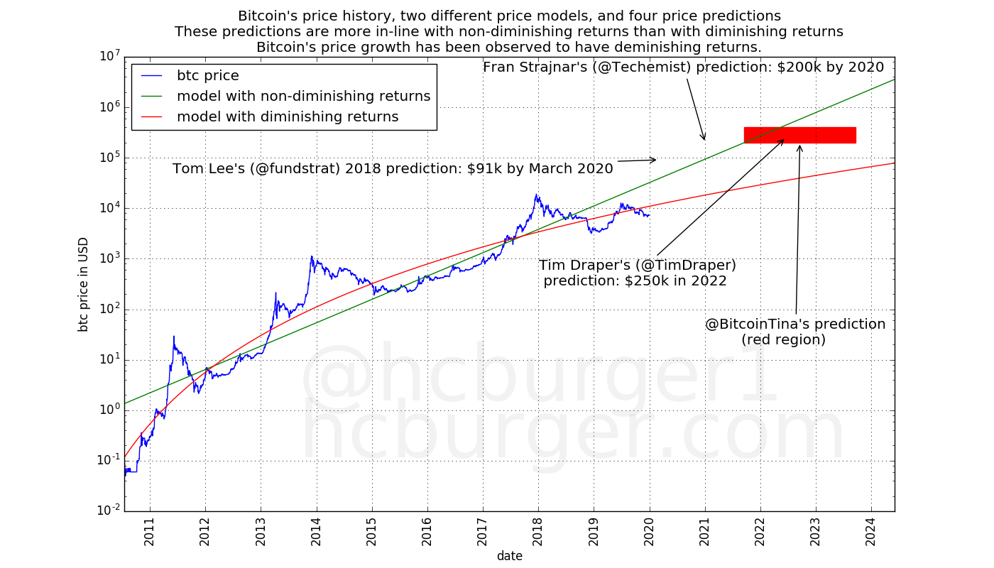
Source of the predictions for Tom Lee and Fran Strajnar, Tim Draper, and BitcoinTina.

Since these predictions are not in line with diminishing returns, and we have empirically observed long-term price growth to be diminishing, it would be surprising for any of these predictions to come true.

Cycle repeats

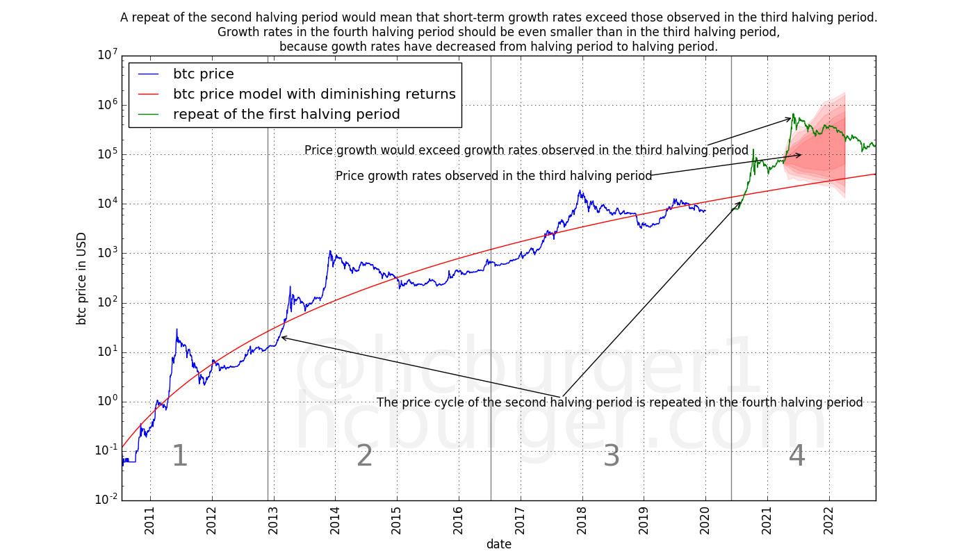
We can also ask ourselves if it is possible for history to repeat itself. E.g. could the price movements observed in the first halving period repeat themselves after the next halving?

For that to be possible, the hypothetical price movements should at least agree with the statistics observed in the third halving period. In fact, we expect the statistics of the price movements in the fourth halving period to be even more tame than those observed in the third period. However, we have not observed any statistics for the fourth having period, so we’re going to work with statistics from the third halving period for now.

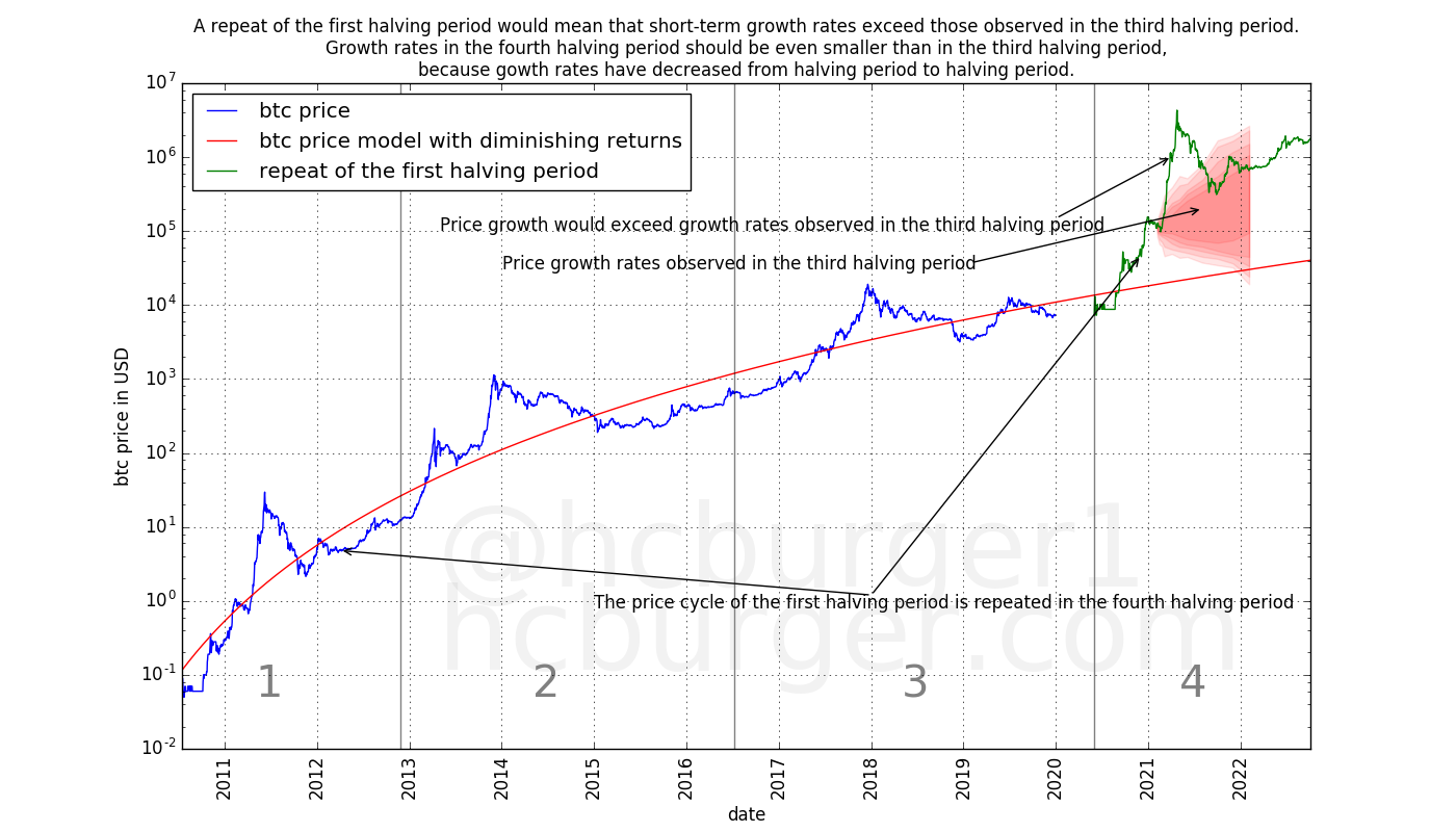
The above plot shows a repeat of the first halving period after the third halving. We see that price movements are too extreme and lie outside the range observed in the third halving period. We should therefore consider a scenario with such strong short-term price fluctuations as unlikely.

What about a repeat of the second halving cycle? The same conclusion holds: the short-term price fluctuations seem to be too strong.

Would a repeat of the third halving cycle be possible? The below plot shows that the price movements are (obviously) in agreement with the statistics observed in the third halving period.

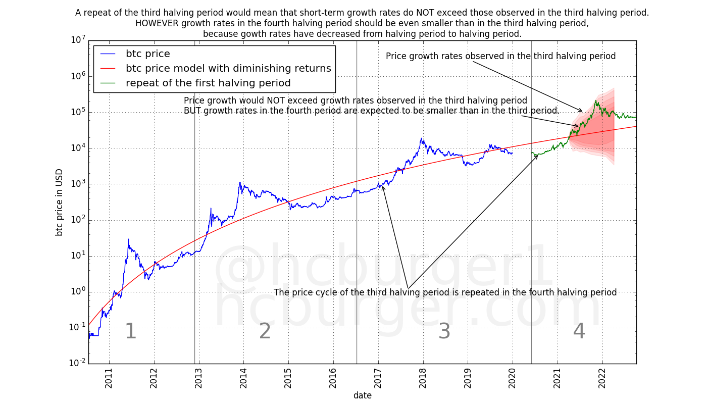
However, short-term price movement statistics should be tamer in the fourth halving period than in the third, for the same reason as statistics in the third period are tamer than in the second period.

We will use a simple method to obtain extrapolated statistics for the fourth halving period, and compare the price movements of the third halving period to those statistics. The extrapolation method works as follows. For a given statistic, it computes the reduction factors from: 1) the first halving period to the second halving period and 2) the second to the third halving period. This average factor is then used to extrapolate the statistic from the third halving period to the fourth.

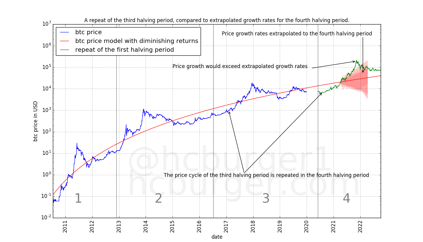
Using this extrapolation method, the price movements of the third halving period would be too extreme.

Assuming 0 price growth until the third halving, and using extrapolated statistics for the fourth halving period, we get the following possible price movements.

Stock-to-Flow model

A model proposed by planB called the stock-to-flow model (S2F for short) models the price of bitcoin using its scarcity, defined as the newly created stock divided by the already existing stock. Price predictions made by this model predict prices in the $100k range for the next halving period, with prices increasing approximately by a factor of 10 for each subsequent halving period:

![](/assets/images/2020/m1/h30.png source: 100trillionUSD

A model which has a constant growth factor (here: 10) for a given period of time (here: 4 years), is a model with non-diminishing returns. Such a model therefore makes claims about the future that are opposed to the observations of long-term diminishing returns we have made in this article, and the expectation expressed in this article that the trend of diminishing returns should continue.

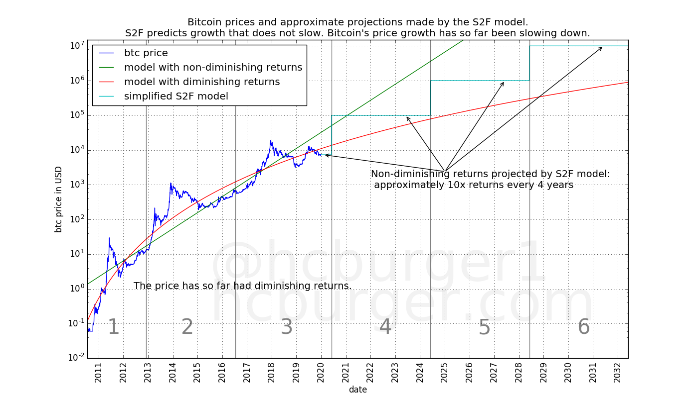
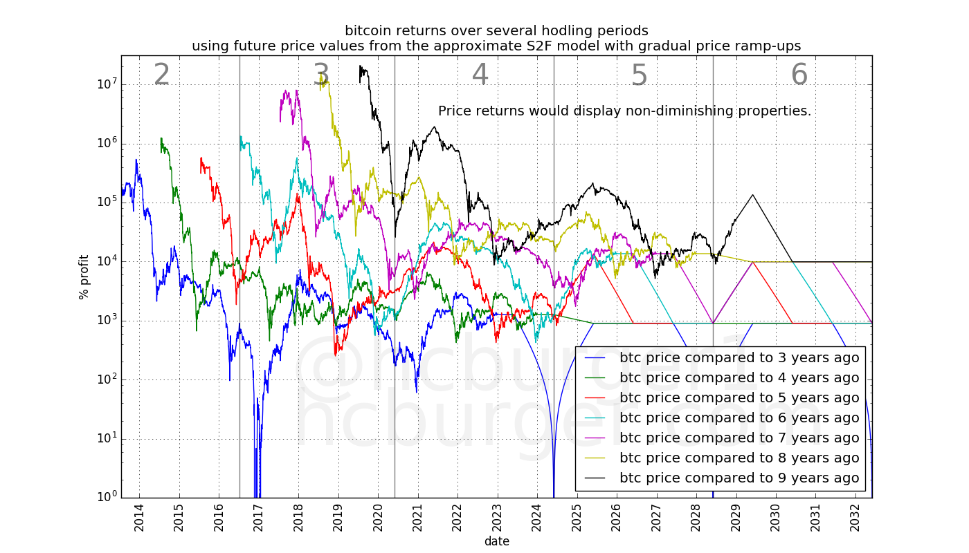
In the short-term, we should not expect the price to move in a step-wise function as displayed by the cyan line (nor does the S2F model claim that the price should evolve in such an abrupt manner). As an experiment, let us consider the following smoother hypothetical future price curve:

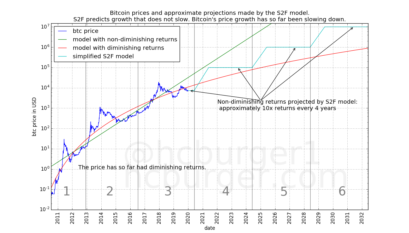
Looking at the return curves that such a price curve would generate, we see that returns at the beginning of the future halving periods (4, 5, and 6) tend to increase. Increasing returns can happen, due to volatility in the price, but should not be expected to happen systematically. We also see that returns for e.g. the three- and four-year hodling periods are more or less flat, at 1000%, reflecting the 10x price increase between halving periods predicted by the S2F model.

Overlaying the return curves generated by the model with diminishing returns shows these disagreements more clearly:

• The S2F model has return curves that are partially increasing, which is not expected in the model with diminishing returns
• The S2F model has return curves that are mostly flat for shorter hodling periods, which indicates non-diminishing returns, whereas in this article we have observed historically diminishing returns.

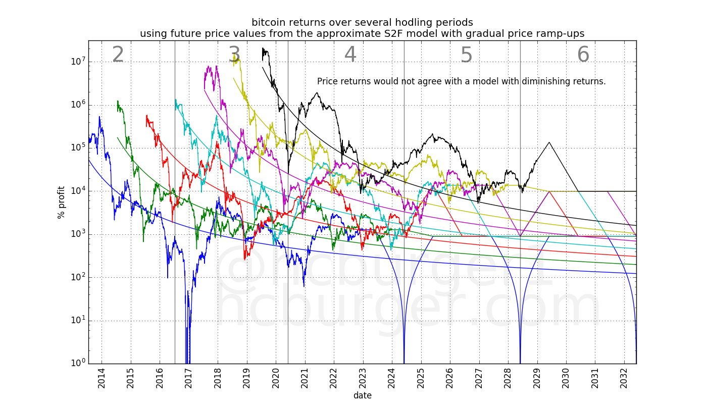
This is not a statement that the S2F model is incorrect, but it does show that for the S2F model to hold as currently formulated, return curves need to change compared to how they have behaved up to now: they need to transition from being diminishing to being non-diminishing.

Also, it is not quite correct to say that the S2F model has non-diminishing returns: In the early history, returns as modeled by the S2F model are indeed diminishing. The returns only diminish up to a certain point, though (approximately a 10x return every 4 years).

The future is still bright

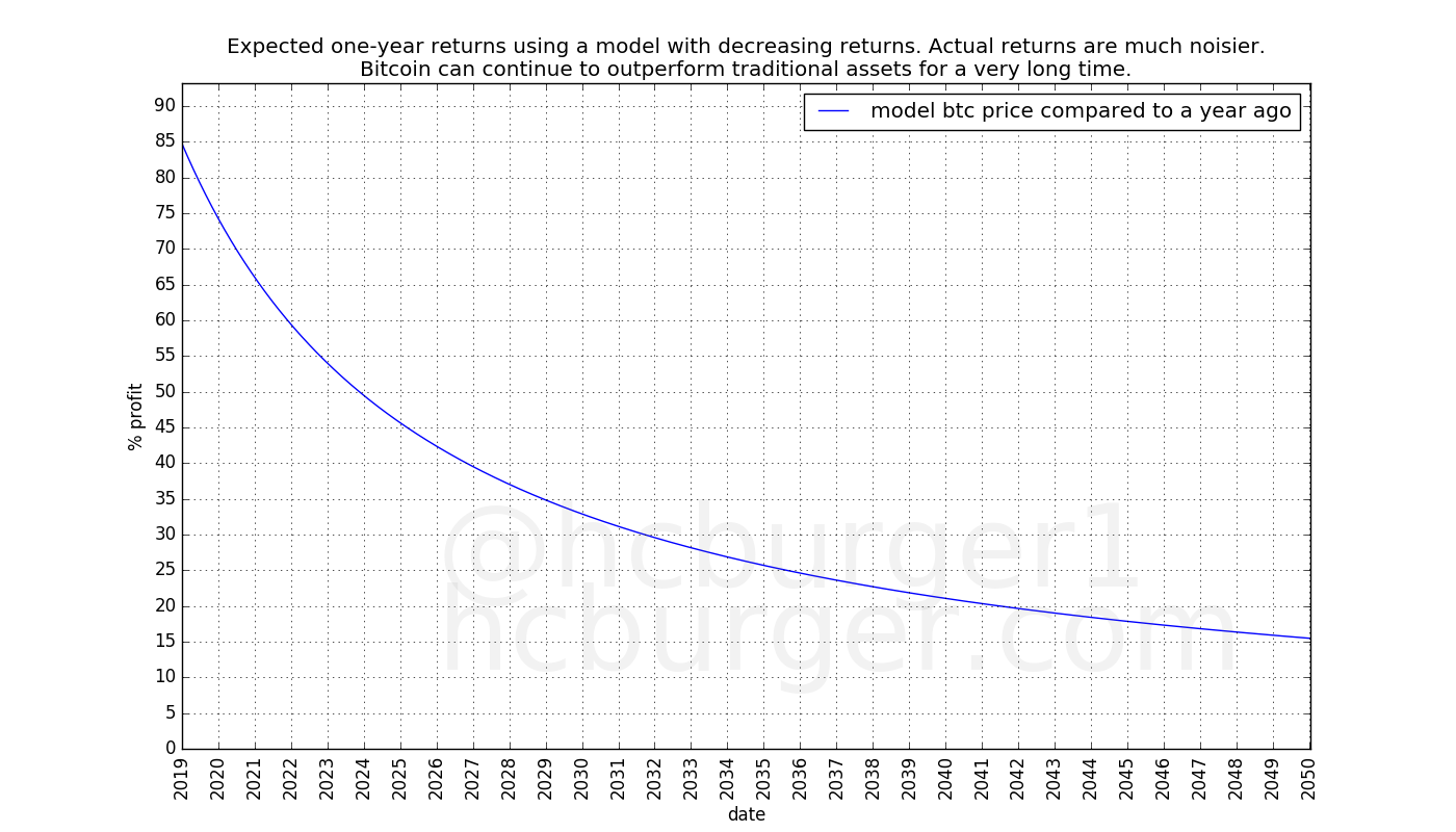
Even though diminishing returns lead to predictions that are less optimistic than predictions based on non-diminishing returns, bitcoin can still have very strong growth for many years to come, and continue to outperform most traditional assets.

Discussion

What this article does not state

This article has made no numerical predictions. No predictions are made regarding the rate of decrease of the long-term price growth rate. Also, no prediction has been made regarding how much volatility is expected to decrease in the future. No statement has been made regarding whether both should tend toward 0 or not.

Potential counter-arguments

Bitcoin’s price growth has at various times been described as being either:

• constant,
• accelerating, or
• resembling an S-curve.

We see no empirical evidence for any of the above. Bitcoin’s price growth has been diminishing from the start.

Why would this property not hold anymore? One might argue that past performance is not an indication of future performance, and therefore that the fact that bitcoin’s returns have so far been diminishing does not mean that they will continue to be diminishing in the future. In other words: bitcoin’s returns could become non-diminishing in the future. As arguments against this statement we can say that:

• We have so far seen no sign that bitcoin is starting to show non-diminishing returns.
• A new, as of yet unknown, mechanism would need to take hold in order to counteract the fact that it becomes ever more difficult to attract ever more capital.

Reasons for slowing growth

We have stated that an increased price of bitcoin leads to more capital being required for even more price increases. We took a shortcut in that explanation: What matters is not only the price, but also the number of bitcoins traded. If few bitcoins are traded, other things being equal, the price of these bitcoins is easier to change than if many bitcoins are traded. One could therefore say that the depth of orderbooks (in fiat terms) really matters, rather than the price itself. So far, orderbook depth has increased along with price.

An alternative way of looking at diminishing returns is the following. The price of bitcoin depends on supply and demand, like anything else. The supply is driven by the willingness of hodlers to part with their bitcoin for a given price. Initial investors were unwilling to part with their bitcoin for anything less than very high returns. These initial sky-high returns attracted more investors, some of which are willing to part with their bitcoins for lower returns (“good enough” returns).

Mathematically, bitcoin’s price growth does not display memorylessness. Memoryless growth would mean that price growth does not depend on its price, which would mean non-diminishing growth. Memoryless/non-diminishing growth would be very surprising, as it would mean that bitcoin’s price has no effect at all on its expected growth rate. We should therefore not expect non-diminishing returns in bitcoin’s price growth, nor do we observe it empirically.

It is also not clear if higher price / deeper orderbooks is the only factor reducing price volatility in the short term. Another reason for reduced volatility might simply be time itself: as time goes by, traders find more and more profitably exploitable patterns. Exploiting these patterns leads to reduced volatility. Yet another reason might be the number of bitcoin traders. The more traders attempt to exploit patterns, the more stable the price is expected to be.

Conclusion

Bitcoin’s price has faced increasing resistance when moving upwards, leading to diminishing returns. Long-term, the price has grown slower and slower. Short-term, volatility has decreased, and bull markets have taken longer to develop and pop. These observations agree with the logic that as the price of bitcoin increases, price movements require ever more capital. For this reason, these two trends are expected to continue in the future. If these trends continue into the future, it will invalidate predictions and models that are based on expectations of non-diminishing returns, which will prove to be too optimistic.

Disclaimer: This article is not financial advice.

---

Related work / Prior art

I am deeply grateful, and also apologetic, to dave the wave, for pointing out to me that he observed both long- and short- term diminishing growth patterns in bitcoin for more than a year.

In a first article, Dave noted:

“As Bitcoin becomes more liquid, it becomes less volatile. Given the principle of the growth curve, this increasing price stability should incrementally come into fruition, with subsequent cycles, as the real volatility of those cycles diminish. These subsequent cycles also see the law of diminishing returns coming into effect though at this relatively early stage of the curve, future returns are projected to remain on quite a different scale to that of traditional asset classes.”

In a later article, Dave noted:

“And this is something you’d expect in a maturing, more liquid market — the general principle being that with more liquidity, comes less volatility. Also predictable, on the basis of the log growth curve model, is a longer base than previously — not only is volatility in the medium term reducing [hence a less volatile base], but so too is volatility reducing on the over-all long-term macro chart of Bitcoin.”

The similarities in the conclusions in Dave’s and this article are striking.

Acknowledgements

This article was inspired by two independent discussions I had. Once with BitcoinEcon, who was pondering whether future bull markets might span longer timeframes than previous ones. This discussion led me to the idea of inspecting short-term growth rates in the various halving cycles. The other with InTheLoop, in which we were discussing how much faith one can really put into any predictive model. This led me to the idea of seeing how far we can go without any model.

Thanks IntheLoop and BitcoinEcon for the great discussions!

Follow me on Twitter

---

Subscribe to WORDS

* indicates required

Email Address *

First Name or Nym *