Stock-to-Flow Influences on Bitcoin Price
| If you find WORDS helpful, Bitcoin donations are unnecessary but appreciated. Our goal is to spread and preserve Bitcoin writings for future generations. Read more. | Make a Donation |
Stock-to-Flow Influences on Bitcoin Price
Challenging the popular understanding
By Nick
Posted March 27, 2020
Abstract
This article attempts to completely invalidate the statistics behind the idea that there is any stock-to-flow relationship to Bitcoin price. The proposed Ordinary Least Squares (OLS) model is shown to be seriously deficient due to the serial correlation in the residuals. The Engle-Granger method is shown to be not usable as a test for cointegration due to requirements for the test not being met. The Johansen method is similarly invalidated. Finally, an Auto Regressive Distributed Lag model (ARDL) is built to test for cointegration. The ARDL model does not falsify the stock to flow relationship. Thus whilst many tests have been able to be shown to be incorrect or have series errors, we have been able to reject the hypothesis that stock-to-flow does not have an important non-spurious influence on the US dollar price of Bitcoin.
Notes
- All analysis was performed using Stata 14.
- This is not financial advice.
Notation
Medium is relatively limited for mathematical notation. The usual notation for an estimate of a statistical parameter is to place a hat on top. Instead, we define the estimate of a term as [ ]. e.g. the estimate of β = [β]. If we are representing a 2x2 matrix, we will do so like this [r1c1, r1c2 \ r2c1, r2c2] etc. Subscripted items are superseded by @ — eg for the 10th position in a vector X we would normally subscript X with 10. We will instead write X@10.
Introduction
Scientific method is difficult for most to comprehend. It is counterintuitive. It can lead to conclusions that do not reflect personal beliefs. It takes a foundation in the method to understand this basic fundamental concept: it is ok to be wrong. This should be something that is taught in school. If we are afraid of getting it wrong, we will never propose anything new. The history of scientific discovery is therefore by its’ very nature surrounded in serendipity. Things that people discover by accident can be just as important as (or more important than) whatever it is they originally set out to do. Their original ideas might have been incorrect or inconclusive, but the things they discovered on the journey built the framework for those who follow.
According to the great modern scientific philosopher Karl Popper, testing a hypothesis for an incorrect outcome is the only reliable way to add weight to the argument that it is correct. If rigorous and repeated tests cannot show that a hypothesis is incorrect, then with each test the hypothesis assumes a higher likelihood of being correct. This concept is called Falsifiability. This article aims to falsify the statistical analysis used thus far to verify the stock-to-flow model of Bitcoin value, as defined in Modelling Bitcoin’s Value with Scarcity[14].
Defining The Problem
To falsify a hypothesis, first we must state what it is:
Null Hypotheses (H0): Stock to flow does not have a measurable influence on Bitcoin price
Alternative Hypotheses (H1): Stock to flow does have a measurable infuence on Bitcoin price
Readers of the first article in this series[3] will note that we have swapped around the null and alternative hypothesis. Readers will also note we are looking specifically at price, not market cap.
In [14], PlanB chose to test H0 by fitting an Ordinary Least Squares (OLS) regression on the natural log of the market capitalisation of Bitcoin and the natural log of the stock-to-flow. There was no accompanying diagnostics nor any identified reasoning for the log transformation in both variables, other than the idea that a log-log model can be expressed as a power law. The model did not take into account the possibility of a spurious relationship due to non-stationarity.
In [3] we explored some alternative models, including ones that do account for the possibility of a spurious relationship. We tested carefully stock to flow and price with both DFGLS and KPSS tests to verify from both directions that both variables were in fact non-stationary. However, the stock to flow variable is not something uninfluenced by the halving events, where the “flow” is literally cut in half. This is more akin to a structural break, rather than a non-stationary increase. Thus we test each halving period’s stock to flow for stationarity with the DFGLS and KPSS test, as well as the entirety of the variable with the Ziffer-Andrews test for stationarity (which was developed to deal with such structural breaks).
Ordinary Least Squares (OLS)
Ordinary least squares regression is a way to estimate a linear relationship between two or more variables.
First, let us define a linear model as some function of X that equals Y with some error.
Y = βX+ε
where Y is the dependent variable, X is the independent variable, ε _is the error term and _β _is the multiplier of _X. The goal of OLS is to estimate β such that ε is minimised.
In order for [β] to be a reliable estimate, some basic assumptions must be met:
- There is a linear relationship between the dependent and independent variables
- The errors are homoscedastic (that is — they have a constant variance)
- The error is normally distributed with a mean of zero
- There is no autocorrelation in the error (that is — the errors aren’t correlated with the lag of the errors)
In the first article of this series [3] we tested the first three of these assumptions. We will now test the fourth — that is how bad is the serial correlation in the residuals (and can we fix it?)
Serial Correlation in the Residuals
We begin by looking at a scatter plot matrix of the lags of the residuals. Serial correlation will show up here as essentially a straight line from the lower left corner of each individual graph to the upper right corner.
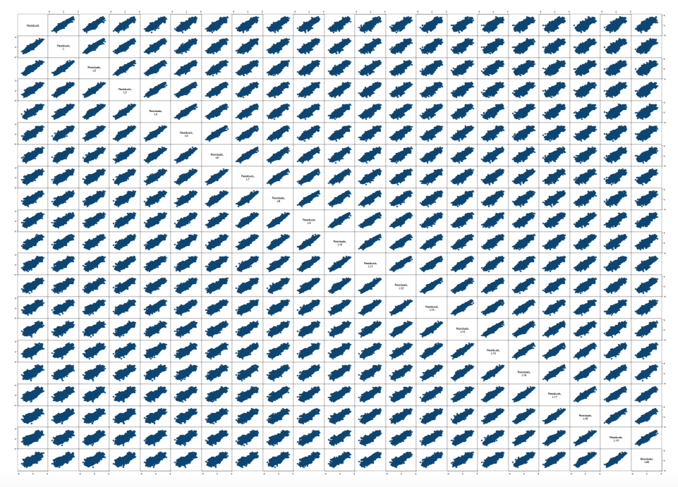 Figure 1 — Scatter plot matrix of Residuals v Lags of Residuals — High correlation shown all the way back to 20 lags
The visual evidence in figure 1 is quite damning. There is serial correlation heavily present. We can confirm this with the Breusch-Godfrey test. The null of the test is no autocorrelation present.
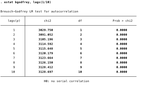 Figure 2 — Breush-Godfrey test for autocorrelation — can reject the null with a high degree of confidence.
We can reject the null in Figure 2 for all lags in the test. This confirms our visual inspection results of autocorrelation in the residuals.
Prais-Winsten regression
Prais-Winsten regression assumes the residuals follow an AR(1) process and accounts for it via the “rho”. Below, we can see the original OLS in figure 3 and the Prais regression in figure 4. In figure 4, we also see the values of the Durbin-Watson statistic — first for the unchanged OLS, and then after accounting for serial correlation.
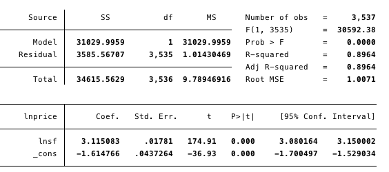 Figure 3 — Original OLS regression results
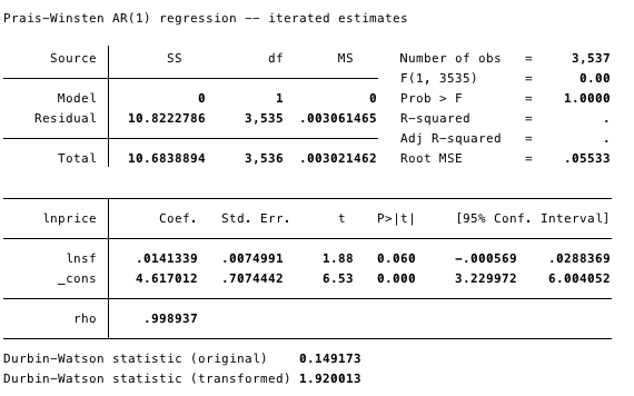 Figure 4 — Prais-Winsten regression results.
Durbin-Watson is for this case interpreted as the closer to 2, the less likely there is to be serial correlation in the residuals.
As we can see, the Prais-Wnisten regression accounts for the serial correlation, however the influence of stock to flow appears greatly diminished, and in fact in this instance, we cannot reject the null hypothesis (that stock to flow does not have an influence on price).
Stationarity
In [1], we used the Johansen test for cointegration. One of the key assumptions in that test (and the simpler Engle-Granger test) is that both variables are non-stationary.
We tested for stationarity in [3] using the DFGLS test and the KPSS test and concluded that both variables were non-stationary. However, conceptually it can be seen that the halving events are more like structural breaks in the stock to flow variable. Thus here we test for stationarity using those tests within the halving epochs.
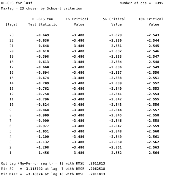 Figure 5 — first halving epoch
We can conclude for the first epoch, that there is insufficient evidence to reject that stock to flow is non-stationary.
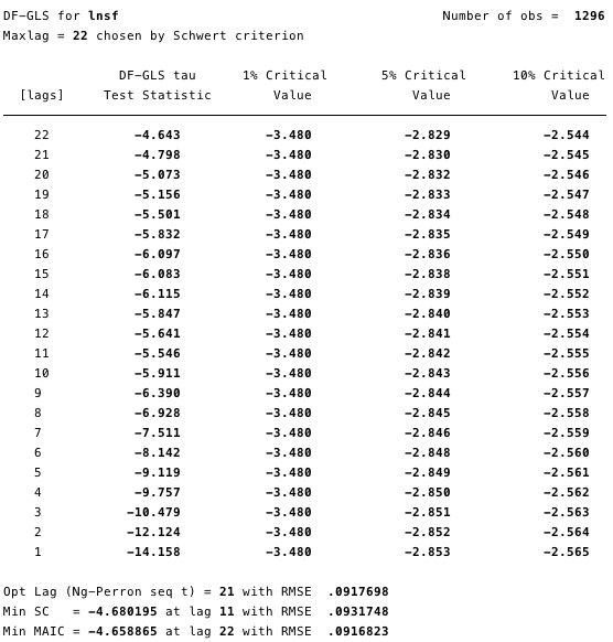 Figure 6 — second halving epoch
For the second epoch, the evidence is more clear — the stock to flow variable is definitely stationary for the second epoch.
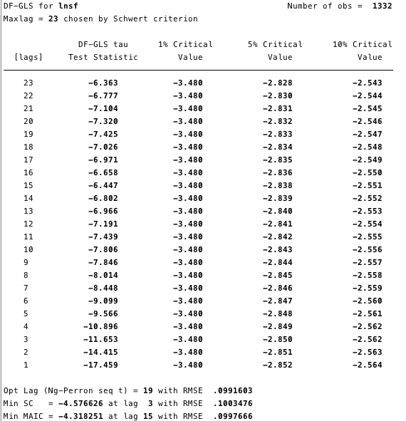 Figure 7 — third halving epoch
In the third epoch, the evidence is overwhelming that stock to flow is stationary. There appears to be a trend toward stationarity through the epochs.
The Zivot-Andrews test for unit root allows for structural breaks in the series, which conceptually aligns with how the halvings impact the flow (and consequently the stock to flow ratio).
Zivot-Andrews unit root test for lnsf
Allowing for break in intercept
Lag selection via TTest: lags of D.lnsf included = 7
Minimum t-statistic -10.081 at 27may2011 (obs 875)
Critical values: 1%: -5.34 5%: -4.80 10%: -4.58
Clearly the Zivot-Andrews test works well here and agrees with the broken down DFGLS tests.
Log(Stock to Flow) is stationary. I(0). This would be fantastic news if Log(price) was also stationary (it would mean the original OLS PlanB did was valid), however it is non-stationary — the Zivot-Andrews test cannot the null.
Zivot-Andrews unit root test for lnprice
Allowing for break in intercept
Lag selection via TTest: lags of D.lnprice included = 7
Minimum t-statistic -3.644 at 16jan2013 (obs 1475)
Critical values: 1%: -5.34 5%: -4.80 10%: -4.58
In [3], we naively assumed stock to flow was integrated order (1) and price was integrated order (1). However, these test show that stock to flow is integrated order (0) and price is integrated order (1).
The Johansen test was used to test for cointegration in [3] — the problem is, we cannot mix orders of integration in this test. We cannot mix them in the simpler Engle-Granger test, either. There is only one possible test that the author is aware of that can deal with mixed order integration — the ARDL bounds test.
Auto Regressive Distributed Lag (ARDL) Model
Autoregressive distributed lag (ARDL) models regress the dependent variable on its lags and on the lags of one or more additional regressors.
ARDL models can, among other things, be used for the estimation and testing of level relationships. Key contributions in this area are [12] and [13]. For a succinct exposition of ARDL models in the context of cointegration, see [5 & 6].
An important feature of the ARDL model is it allows us to investigate relationships between mixed orders of integration.
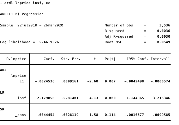 Figure 8 — ARDL model on daily data. We can see stock to flow has a significant long run influence on price.
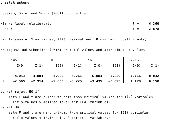 Figure 9 — Bounds test for a level relationship. We can reject the null hypothesis of no level relationship easily at the 10% critical level, further providing evidence to the s2f claim (NB we are looking at the I(0) variable s2f).
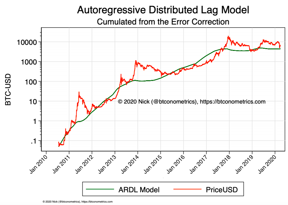 Figure 10 — Showing the long-run (LR) influence of stock to flow on price
Discussion
The bounds test for a level relationship in the ARDL model provides very robust evidence to reject the null hypothesis and conclude that stock to flow does have a significant influence on the US Dollar price of Bitcoin.
Further research is required as the coefficient for the long run parameter is significantly lower than the OLS parameter. Future research should focus on improving the ARDL specification, including adjusting for confounding or potentially effect mediating variables (such as the difficulty adjustment).
Follow me on twitter: @btconometrics or visit my website: https://btconometrics.com for further information.
Citations and Further Reading
- Popper, Karl (1959). The Logic of Scientific Discovery (2002 pbk; 2005 ebook ed.). Routledge. ISBN 978–0–415–27844–7
- Murray, M. (1994). A Drunk and Her Dog: An Illustration of Cointegration and Error Correction. The American Statistician,48(1), 37–39. doi:10.2307/2685084
- Nick. (2019), Falsifying Stock-to-Flow As a Model of Bitcoin Value — The Drunken Value of Bitcoin, btconometrics.com — https://medium.com/swlh/falsifying-stock-to-flow-as-a-model-of-bitcoin-value-b2d9e61f68af
- Dickey, D. A. and W. A. Fuller (1979). Distribution of the estimators for autoregressive time series with a unit root. Journal of the American Statistical Association, 74 (366), 427–431.
- Hassler, U. and J. Wolters (2006): Autoregressive Distributed Lag Models and Cointegration. Allgemeines Statistisches Archiv, 90, 59–74.
- Hassler, U. and J. Wolters (2005): Autoregressive Distributed Lag Models and Cointegration. Freie Universitaet Berlin, Working Paper №2005/22.
- Kripfganz, S. and D. Schneider (2018): Response Surface Regressions for Critical Value Bounds and Approximate p-values in Equilibrium Correction Models. Manuscript, University of Exeter and Max Planck Institute for Demographic Research. Available at www.kripfganz.de/research/Kripfganz_Schneider_ec.html.
- Luetkepohl, H. (2005): New Introduction to Multiple Time Series Analysis. Berlin, Heidelberg: Springer Verlag.
- MacKinnon, J. G. (1991). Critical values for cointegration tests. In: R. F. Engle and C. W. J. Granger (Eds.): Long-Run Economic Relationships: Readings in Cointegration, Chapter 13, pp. 267–276. Oxford, UK: Oxford University Press.
- MacKinnon, J. G. (1996). Numerical distribution functions for unit root and cointegration tests. Journal of Applied Econometrics, 11 (6), 601–618.
- Narayan, P.K. (2005): The Saving and Investment Nexus for China: Evidence from Cointegration Tests. Applied Economics, 37 (17), 1979–1990.
- Pesaran, M.H. and Y. Shin (1999): An Autoregressive Distributed Lag Modelling Approach to Cointegration Analysis. In: Strom, S. (Ed.): Econometrics and Economic Theory in the 20th Century: The Ragnar Frisch Centennial Symposium. Cambridge, UK: Cambridge University Press.
- Pesaran, M.H., Shin, Y. and R.J. Smith (2001): Bounds Testing Approaches to the Analysis of Level Relationships. Journal of Applied Econometrics, 16 (3), 289–326.
- PlanB. (2019) Modelling Bitcoins Value with Scarcity. https://medium.com/@100trillionUSD/modeling-bitcoins-value-with-scarcity-91fa0fc03e25