Reviewing “Modelling Bitcoin’s Value with Scarcity” — Part IV: The Theoretical Framework leading to the Error Correction Model
| If you find WORDS helpful, Bitcoin donations are unnecessary but appreciated. Our goal is to spread and preserve Bitcoin writings for future generations. Read more. | Make a Donation |
Reviewing “Modelling Bitcoin’s Value with Scarcity” — Part IV: The Theoretical Framework leading to the Error Correction Model
The next step after the shown cointegrating relation between stock-to-flow and market cap of bitcoin
By Marcel Burger
Posted March 7, 2020
Introduction
In my first review of the work of PlanB, I concluded that the relation between stock-to-flow and bitcoin price as pointed out by the author was invalid because the general assumptions of ordinary least squares regression were not met. When two variables are non-stationary and we estimate a regression model, there is a good chance we find highly autocorrelated residuals and a significant value for the coefficient. This phenomenon is well known as spurious regression. But, spurious regression isn’t always the case. Sometimes the variables might be cointegrated, which would imply that the estimated relation is super consistent. Nick pointed out that we could very well be dealing with the exceptional case of cointegration and showed that he wasn’t able to falsify the cointegrating relationship between stock-to-flow and bitcoin’s market cap. After Nick showed that the variables were cointegrated, I verified his findings. Since I still was skeptic, I chose to run the analysis on my own dataset and ran three different cointegration tests to make sure there was no doubt. Even though I expected I would be able to show that at least one of those tests would lead me to reject cointegration, I could not. Initially, I was a bit too fast with drawing my conclusions and as a result I warned people that the model was flawed. So, I offered my apologies in public for drawing a wrong conclusion and engaged in many discussions to explain why the model was eventually right. Because I noticed in those discussions that the basis underneath the material we discuss is poorly understood by most people, I decided to start writing a book that will help people to better understand the econometric concepts we’re dealing with. To stay in the loop about that development, I recommend subscribing at www.bitcoinometrics.io to get notified once the book is available. But that’s not what this piece is about. This piece is about further development of the model and presenting a framework which helps to understand the developments. In the process of writing my book I also conduct some academical research. Not only to refresh my mind on time series analysis, but also to check with academical researchers if there were any important developments in that field of research. Nick in his write up already mentioned the Vector Error Correction Model (‘VECM’) and estimated the coefficients for the model as part of his attempt to falsify cointegration. In my ‘hunt for cointegration’ I also touched on it without estimating any of the model coefficients, but I ended the article by stating that setting up a VECM would be a nice subject for a follow up article. This is still work in progress, but I like to share a bit more on how we actually get to that point and how to go about.
Model Selection Framework
Usually when one is looking to quantify the relation between non-stationary time series, the first step is to difference the series until a stationary series is found. This is basically the first thing you learn as an Econometrics student when you follow classes on Regression Analysis or Time Series Analysis. But differencing the time series to make them stationary is only one possible direction to come to a solution. And it comes at the cost of throwing away data that might identify long run relationships between the time series.
Another possibly better solution is to test whether the time series are cointegrated. If the cointegration test tells us cointegration exists, we can set up a model that is able to describe both the long run relationship and the short term corrections.
One of the things I noticed in the literature is that it’s hard to find a basic method selection decision tree. I like to attack these kind of problems as structured as possible, so that the chance of actually finding meaningful relations increases while you also prevent yourself from misspecifying a model. In my search for a helpful framework, I found this useful article.
The framework as shown below is my slightly adjusted version that is based on the one I found. It will serve as a guide in the steps we will take. All the shapes that contain bold text, show the path we follow in case we like to construct a model to quantify the relation between stock-to-flow and price (or market cap). In the earlier articles (here and here) Nick and I both independently showed that both variables are first order integrated (after applying differencing we end up with a stationary series over time) and that cointegration couldn’t be rejected by running different tests.
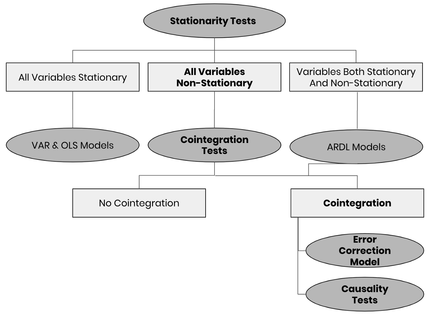 Fig 1: Simplified Model Selection Framework for time series analysis
Note that even though the overview above is far from complete, it offers a useful overview for those models that are often used. Most practitioners who use linear regression models, just go straight to the OLS models without even testing for stationarity. Using frameworks like these would be beneficial to many of them. It also helps people with less of a statistical background to check whether the beautiful model they have been introduced to was indeed the appropriate model to use.
Please also note that this overview is only about model selection and not about estimation of the model. I like to emphasise again that this overview is very simplified.
We found cointegration. Now what?
As cointegration couldn’t be falsified, this means that the two variables are linked to form an equilibrium relationship spanning the long run. One of the issues though with the different cointegration tests is that some of them have weaknesses. Johansen (1988) addressed those and came up with an improved cointegration test model, which is widely applied nowadays and incorporated in many different econometric software packages. Both Nick and I used that test in our model validation and we concluded that the model as introduced by PlanB couldn’t be falsified.
If both the variables are first order integrated and there exists a cointegration relationship then we can derive an Error Correction Model. When both variables are put into a vector this can also more generally be referred to as a Vector Error Correction Model (‘VECM’).
Following the framework
First, I set up all the different equations, and briefly touch upon them. Keep in mind that the long term relation is what matters most in terms of showing us the road, and realise that the short term corrections are modelled to return to the middle of the road. In order to run a full blown analysis we need to define:
- the linear model
- the cointegration representation
- the error correction models for both S2F and BMC
- the models to run causality analysis
Setting up the model equations
If we consider the logarithm of bitcoin market cap (‘Log(BMC)’) as _Y _and we consider the logarithm of stock-to-flow (‘LogS2F’) as _X, _then the relationship between the two is written as:
 Equation 1: The Linear Model
Based on the representation theorem of Engle and Granger (1987), we rewrite the equation to display the cointegrating relationship:
 Equation 2: Cointegration Representation
Since both variables have their own Error Correction Models, I introduce them here:
 Equation 3: Error Correction Model for bitcoin market cap
 Equation 4: Error Correction Model for Stock-To-Flow
The first expressions at the right hand side of the Error Correction Model equations indicated by ⍺ are both stationary white noise processes for some number of lags _l. _In case we look at only at one period lag, the equations become:
 Equation 5: Error Correction Model for BMC with one lag.
 Equation 6: Error Correction Model for S2F with one lag
The coefficients in the cointegration equation are used to show the estimated long term relation among S2F and BMC. The coefficients in the Error Correction Models will provide more information on how deviations from that long term relation affect the changes on them in the next period. In this case 𝜌 measures the speed of adjustment to the long term equilibrium. So, when the model runs away from the long term theoretical price, these coefficients tell us how fast we will return to it.
It’s important to note that all equations above on their own, are just equations. I preferred to keep it readable, by not addressing the assumptions over and over again. In order to turn these equations into models we should say something about what assumptions are made regarding the errors. In case we like to use parametric estimation we have to either use ‘the weak’ or ‘the strong’ assumptions regarding the error. Under the weak assumptions we only make assumptions regarding the first 2 moments of the distribution, while under the strong assumption we define the entire distribution itself.
Causality Testing and required models
Since S2F and BMC are cointegrated, one of the following statements regarding this relationship will hold:
- S2F drives BMC,
- BMC drives S2F,
- or BMC and S2F drive each other
If S2F and BMC were not cointegrated, there would be no causal relation and the two variables would be independent. Granger (1969) has developed a causality test method that will enable us to determine the direction of the relationship. If current and lagged values of S2F improve the prediction of the future value of BMC, then it is said that S2F Granger causes BMC. And the opposite can be said as well.
The model equations that we build to test for the direction of the relation are shown below:
 Equation 7: Model to test if X Granger causes Y
 Equation 8: Model to test if Y Granger causes X
In both cases we are testing the null hypothesis that beta and delta are equal to zero. If beta in equation 7 is equal to zero then X is not Granger causing Y (or LogS2F is not Granger causing LogBMC). And in equation 8 we test for delta being equal to zero.
Estimating the model coefficients
In order to estimate model coefficients we can either choose between parametric or non parametric approaches or some kind of combination of both. As stated by Green:
“Contemporary econometrics offers the practitioner a remarkable variety of estimation methods, ranging from tightly parameterized likelihood based techniques at one end to thinly stated nonparametric methods that assume little more than mere association between variables at the other, and a rich variety in between. Even the experienced researcher could be forgiven for wondering how they should choose from this long menu.” As a general proposition, the progression from full to semi- to non-parametric estimation relaxes strong assumptions, but at the cost of weakening the conclusions that can be drawn from the data.
The main reason to use a parametric estimation is that we can infer stronger conclusions (as long as assumptions are respected), because we use strong assumptions w.r.t. the distributions of the variables we analyse. At the other hand, the advantage of non parametric estimation is that we don’t need to impose strong assumptions on the distributions of the variables we analyse, but we can just go with their actual distribution. As long as the actual distribution comes close enough to the imposed distribution, I would prefer to go with parametric estimation (like OLS estimation), but when the imposed distribution is not really a good match with the actual distribution, non-parametric estimation is preferred.
What’s next?
I intended to write a piece on the estimation of the VECM model coefficients, but actual estimation calculations are put on the ToDo list for now. This piece has been in draft mode for a while, so I decided to split up the content into a theoretical part and a more hands on estimation of the parameters. So, next in line is running some actual calculations on different estimation techniques and presentation of the results.